Emergent Behavior of a Structured Vacuum
A constructive effective-field framework that treats the vacuum as a continuous medium with displacement, local rotation (tetrad), and scale. In the appropriate limits: shear reproduces Einstein–Hilbert gravity, twist yields Maxwell electrodynamics, and scale produces a Bergmann–Wagoner scalar–tensor sector—while enabling additional medium-induced interactions (e.g., birefringence and light-by-light scattering) and a spin–quadrupole channel for gravitational radiation.
Key Claims
- Shear-only sector reproduces the Einstein–Hilbert action in the effective limit.
- Twist-only sector yields vacuum Maxwell equations via abelian projection of torsion.
- Scale sector maps to a Bergmann–Wagoner / Brans–Dicke–type scalar–tensor structure.
- Quartic-order terms suggest new testable channels (birefringence, light-by-light scattering, spin–quadrupole GW).
- Open-source simulator released to support reproducibility and exploration of cross-couplings.
Emergent Behavior of a Structured Vacuum
Last Updated: 2025-12-20T00:00:00-08:00
We model the vacuum as a structured medium with three fields: A displacement (shear) \(u^{i}\), an orthonormal frame \(e^{a}{}_{\mu }\) encoding rotations (twist), and a scalar (scale) field \(\sigma \). Using a constructive derivation that removes non-physical couplings, we demonstrate that (i) the shear-only sector reproduces the Einstein–Hilbert action, (ii) the twist-only sector yields Maxwell electrodynamics, and (iii) the scale sector produces a Bergmann–Wagoner scaler-tensor theory. While a structured vaccuum is able to recover familiar physics at effective limits, is also has the potential to support additional medium-induced interactions, including contributions to vacuum birefringence and light-by-light scattering, and a spin-quadrupole channel for gravitational radiation. We release an open-source simulator implementing the model’s dynamics to facilitate reproducibility and to enable exploration of cross-couplings and testable consequences.
1 Why Revisit Empty Space?
In the nineteenth century, physicists pictured an ether—a rigid, all-pervasive substrate that conveyed light yet remained otherwise undisturbed by matter. With special relativity, twentieth century physicists dismissed the ether’s rest frame, and quantum field theory recast the vacuum as the state nullified by all annihilation operators. While these opposing views of the vacuum helped aid the explanation of their respective physical theories, they both suffer from a complementary deficiency: The ether carries too much structure (an absolute rest frame), while the quantum vacuum carries too little.
In this paper, we chart a course for a middle path: A structured vacuum that is material enough to endow space-time with elasticity and spin, yet symmetric enough to satisfy the relativity principle. We argue that observable phenomena arise as emergent behavior governed by the rules of interaction among the medium that comprises the structured vacuum and we show that our framework is flexible enough to encompass a variety of prior theories in the appropriate limits. We also release as open source a simulator that models a discrete version of our framework, which can be used to reproduce our results and as a test-bed for exploring structured vacuum dynamics.
2 Statement of Principles
We begin by establishing two principles that will guide our search for the dynamics that govern the structured vacuum. We develop the rest of our structured vacuum from successive derivation from these first principles.
The differential equations governing the vacuum medium retain the same form in every inertial coordinate system.
No experiment confined to a moving laboratory can reveal its state of motion with respect to the medium. Specifically, the speed of small amplitude elastic or torsional waves that propagate through the medium are isotropic in every inertial frame.
All physical fields are collective excitations of a single continuous medium whose local state is described by
\[ \left [u^{i}(x),\;e^{a}{}_{\mu }(x)\right ], \]
where \(u^{i}\) encodes translations and \(e^{a}{}_{\mu }\) encodes intrinsic rotations.
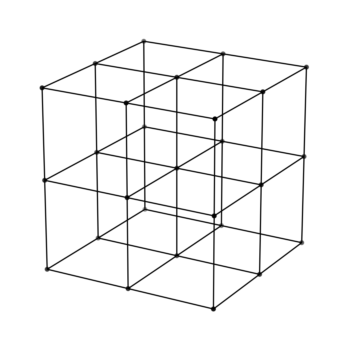
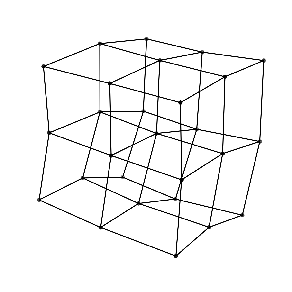
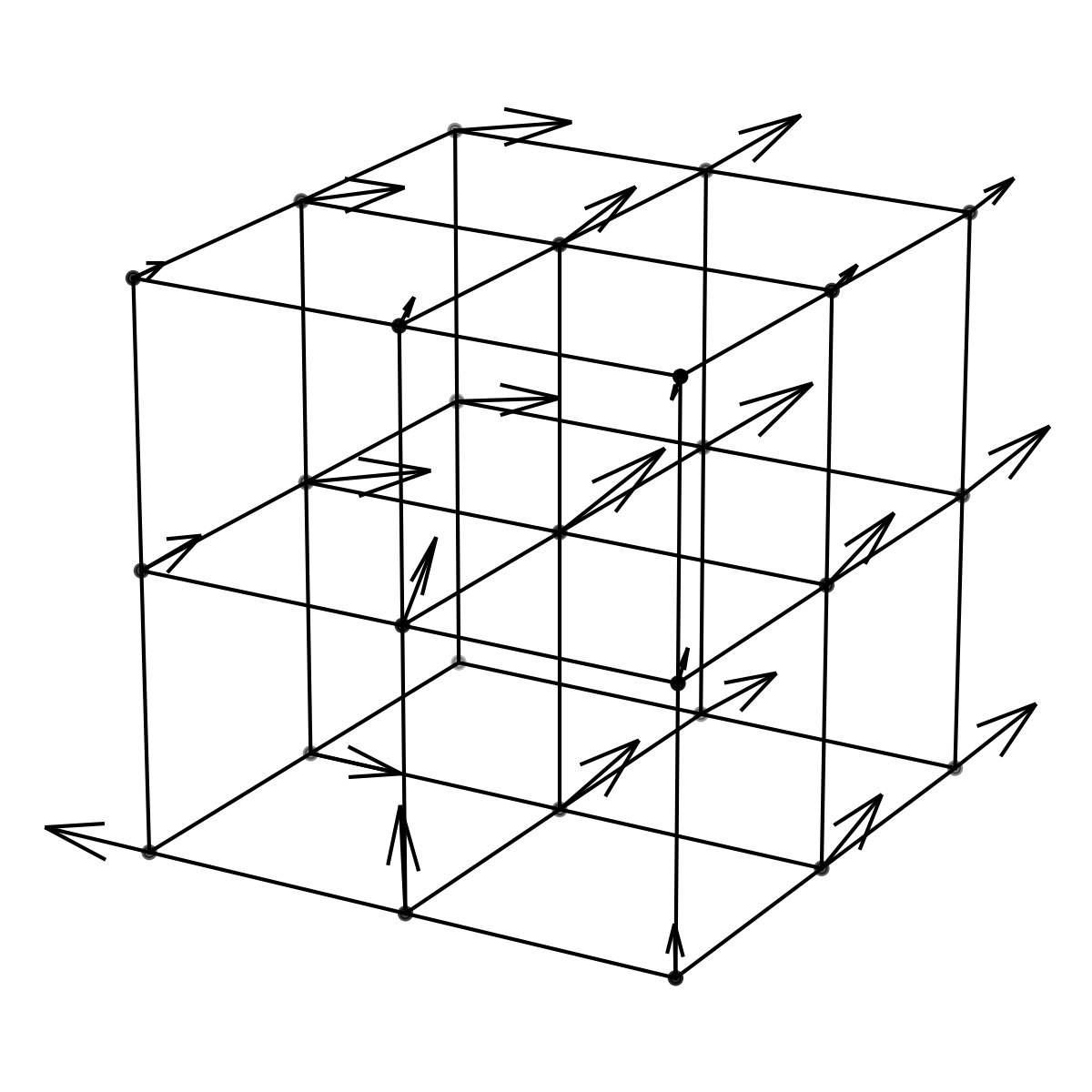
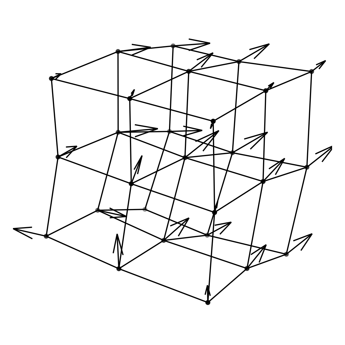
The vacuum combines both elastic translations and torsional rotations in a single substrate. This primitive geometry naturally gives rise to both compressional waves as well as rotational waves without selecting a preferred rest frame. Figure 1 shows a visual representation of some examples of perturbations the structured vacuum medium supports.
Building upon these two principles as a foundation, our goals for the rest of this paper are to (a) find the most economical set of relativistically covariant differential equations obeyed by \(\left (u^{i},\;e^{a}{}_{\mu }\right )\) and (b) to compare their consequences with observation. Section 3 sets the stage by defining the kinematics of the structured vacuum’s inertial system; Section 4 shows how at two derivatives the linearized Einstein equation, the vacuum Maxwell equations, and a Bergmann-Wagoner scaler-tensor theory of gravity emerge; and Section 5 shows how at four derivatives the model adds additional precision to the prior theories with the Einstein–Hilbert action of general relativity and the non-linear Maxwell equations emerging along with other potential cross-terms that indicate the potential for the medium to support vacuum birefringence, light-by-light scattering, and spin–quadrupole gravitational radiation. Section 6 describes the design, implementation, and usage of our open source simulator.
3 Vacuum Geometry and Kinematics
We work in an inertial system \(\mathcal {K}\) with coordinates
\[ x^{\mu } = (t,x,y,z). \]
We use Greek letters to refer to external space-time indices. Material points in the structured vacuum carry labels \(\xi ^{i} = \left (\xi , \eta , \zeta \right )\) and are fixed (Lagrangian coordinates); their world-lines are the maps
\[ Y^{\mu } : \mathbb R^{3}\times \mathbb R \;\to \; \mathbb R^{4}, \qquad (\xi ^{i},t)\mapsto Y^{\mu }(\xi ^{i},t). \]
When raising and lowering indices, we use the Minkowski metric, for example, \(\Lambda _{\mu }{}^{\nu } = \eta _{\mu \nu }\Lambda ^{\nu }{}_{\rho }\eta ^{\rho \mu }\).
It is useful to split the world-line into the identity embedding plus a small deviation:
\[ Y^{\mu }(\xi ,t)\;=\;Y^{\mu }_{0}(\xi ,t)+u^{\mu }(\xi ,t), \qquad Y^{\mu }_{0}(\xi ,t)\;=\;(t,\xi ,\eta ,\zeta ), \]
so that \(u^{i}\) measures the displacement of the labelled point \(\xi ^{i}\) from the reference rest frame.
A local tetrad \(e^{a}{}_{\mu }(\xi ,t)\) attaches an orthonormal basis to each point to record intrinsic rotations relative to its neighboring points,
\[ e^{a}{}_{\mu }(\xi ,t),\qquad e^{a}{}_{\mu }\,e_{a\nu }=g_{\mu \nu },\; e^{a}{}_{\mu }\,e^{b\mu }=\eta ^{ab}. \]
We use Latin letters to refer to the internal material frame indices. Each \(e^{a}\) records how the element is rotated relative to its neighbours. We use the set of material frames attached to each point to form the metric for the observable geometry, \(g_{\mu \nu }\), and ideal flat-space, \(\eta ^{ab}\).
As a matter of bookkeeping for this rotation-based field, we define a translation between local Lorentz gauge and teleparallel gauge. Let \(\omega ^{a}{}_{b\mu }\) denote a flat spin connection, such as,
\[ R^{a}{}_{b\mu \nu }\left [\omega \right ]\;=\;0. \]
Here, \(\omega \) is pure gauge and carries no new dynamics; thus, we have
\[ \omega ^{a}{}_{b\mu }\;=\;\left (\Lambda ^{-1}\partial _{\mu }\Lambda \right )^{a}{}_{b}, \]
for some Lorentz matrix \(\Lambda (x)\). We define,
\[ \mathcal {D}_{\mu }e^{a}{}_{\nu }\;\coloneq \;\partial _{\mu }e^{a}{}_{\nu }+\omega ^{a}{}_{b\mu }e^{b}{}_{\nu }. \]
Without loss of generality—and motivated by our desire to keep our notation tidy—we evaluate covariant derivatives in the inertial gauge, \(\omega ^{a}_{b\mu } = 0\). At any time, we can restore local Lorentz covariance with \(e^{a}{}_{\mu } \mapsto \Lambda ^{a}{}_{b}(x) e^{b}{}_{\mu }(x)\) and the standard transformation \(\omega ^{a}{}_{b\mu } \mapsto \Lambda ^{a}{}_{c}(x) \omega ^{c}{}_{d\mu }\left (\Lambda ^{-1}\right )^{d}{}_{b} + \Lambda ^{a}{}_{c} \partial _{\mu }\left (\Lambda ^{-1}\right )^{c}_{b}\).
The determinant of the tetrad, \(|e|\equiv \det (e^{a}{}_{\mu })=\sqrt {-g}\), is a scalar density of weight \(+1\) under diffeomorphisms: \(|e|'(x')=\left |\frac {\partial x}{\partial x'}\right |^{-1}|e|(x)\). To build a genuine scalar from it we introduce a dimensionless dilaton
\[ \sigma (x)\;\equiv \;\ln \!\frac {|e|(x)}{|e|_{0}}, \]
where \(|e|_{0}\) is a fixed reference density of the same weight (its only role is to make the argument of the logarithm dimensionless). Then \(\sigma \) is a true scalar and \(\nabla _{\mu }\sigma \) is a true vector.
As an example, let \(\mathcal K'\) move with constant velocity \(v\) along the \(x\)-axis of \(\mathcal K\). The standard Lorentz matrix is
\[ \Lambda ^{\mu }{}_{\nu }= \begin {pmatrix} \gamma & -\gamma \beta & 0 & 0\\ -\gamma \beta & \gamma & 0 & 0\\ 0 & 0 & 1 & 0\\ 0 & 0 & 0 & 1 \end {pmatrix}, \qquad \beta =\frac {v}{c},\;\;\gamma =\frac {1}{\sqrt {1-\beta ^{2}}}. \]
The principle of relativity requires that \(u^{\mu }\) transforms as a contravariant four-vector in every inertial frame:
\(\seteqnumber{0}{}{0}\)\begin{equation} \label {eq:u-transform} u'^{\mu }(x') = \Lambda ^{\mu }{}_{\nu }\,u^{\nu }(x), \qquad x'^{\mu }=\Lambda ^{\mu }{}_{\nu }\,x^{\nu }. \end{equation}
Carrying out the matrix multiplication, we get
\[ u'^{0} = \gamma \left (u^0-\beta \,u^{x}\right ),\qquad u'^{x} = \gamma \left (u^{x}-\beta \,u^{0}\right ),\qquad u'^{y}=u^{y},\; u'^{z}=u^{z}. \]
Since the time component \(u^{0}=0\) in \(\mathcal {K}\) by construction, we find that
\[ u'^{0} = -\gamma \beta \,u^{x},\qquad u'^{x} = \gamma \,u^{x},\qquad u'^{y}=u^{y},\; u'^{z}=u^{z}. \]
Thus, time-like components appear in \(\mathcal K'\) even if absent in \(\mathcal K\); they encode the relativity of simultaneity for the stretched vacuum medium. If \(u^{i}\) describes the elastic “stretch” of a material measured at one instant, the boosted observer sees that different parts of the medium have that stretch at different times. The non-zero time component \(u'^{0}\) is the bookkeeping term that encodes when each part of the stretch happens in \(\mathcal K'\).
Similarly, take the tetrad \(e^{a}{}_{\mu }\) in \(\mathcal K\): Under a boost \(\Lambda ^{\mu }{}_{\nu }\) between \(\mathcal K\) and \(\mathcal K'\) the transformation law reads
\(\seteqnumber{0}{}{1}\)\begin{equation} \label {eq:e-transform} e'^{a}{}_{\mu }(x')=\Lambda _{\mu }{}^{\nu }\,e^{a}{}_{\nu }(x), \qquad e'^{a}{}_{\mu }\,e'_{a\nu }=g'_{\mu \nu }. \end{equation}
Only the external space-time slot \(\nu \) transforms while the internal material frame index \(a\) remains inert. Intrinsic orientation belongs to the medium itself, not to the observer. In other words, if the medium is “stretched” in a certain internal direction, every observer must agree which internal axis \(a\) is stretched, but they will disagree on how the axis is decomposed into external space-time coordinates.
Finally, take the determinant of the tetrad, \(|e|\), under a boost \(\Lambda \):
\(\seteqnumber{0}{}{2}\)\begin{equation} \label {eq:det-transform} |e'|\;=\;\det \left (\Lambda _{\mu }{}^{\nu }\,e^{a}{}_{\nu }\right ) \;=\;\det \left (\Lambda _{\mu }{}^{\nu }\right )\,\det \left (e^{a}{}_{\nu }\right ) \;=\;\det \left (\Lambda \right )\,|e|. \end{equation}
For a Lorentz boost, we have \(\det \left (\Lambda \right )=1\), giving us \(|e'|=|e|\). If we allowed a transformation that changed parity or time orientation, we would instead have \(\det \left (\Lambda \right )=-1\), which would cause the boosted determinant \(|e'|\) to pick up a minus sign. Under global Lorentz coordinate transformations the Jacobian has unit determinant, so \(|e|\) is numerically unchanged, but under general coordinate changes it transforms as a density.
The set of rules in Equations (1), (2), and (3) provide us with the complete Lorentz behavior we need to build invariant actions. In the next section, we identify the only set of non-trivial differential equations that obey the principles of relativity and universality.
4 Quadratic Vacuum Dynamics
To give the reader a feel for the way the vacuum is structured, we start with a simplified quadratic action. We build this action from the first principles we define in Section 2 and argue why the geometry of the vacuum must give rise to the terms in the action. In Section 5, we use this same process to derive the full-blown action (at least for the present work) at the quartic order.
The gradient field \(\partial _{\mu }u^{i}\) splits into two parts: A symmetric part representing the strain of the medium, and an antisymmetric part representing the rigid rotation of the medium. We use the symmetric part of \(\partial _{\mu }u^{i}\) to build the effective metric as only the symmetric part changes lengths,
\[ g_{\mu \nu }= \partial _{\mu }Y^{\alpha }\,\partial _{\nu }Y_{\alpha }, \]
where for small displacements, we write
\[ Y^{\alpha }_{0}(\xi ,t)\;=\;(t,\xi ,\eta ,\zeta ),\qquad Y^{\alpha }=Y^{\alpha }_{0}+u^{\alpha },\qquad g_{\mu \nu }= \eta _{\mu \nu }+2\,\partial _{(\mu }u_{\nu )}+\order {u^{2}}. \]
The antisymmetric derivative of the tetrad, \(\partial _{[\mu }e^{a}{}_{\nu ]}\), isolates the piece of the action that cannot be absorbed into a smooth metric change, and supplies torsion,
\[ T^{a}{}_{\mu \nu }=2\,\mathcal {D}_{[\mu }e^{a}{}_{\nu ]}. \]
At the ground state, \(u^{\mu }=0\) and \(g_{\mu \nu }\) reduces to the flat background, \(\eta _{\mu \nu }\); similarly, when \(e^{a}{}_{\mu }=\delta ^{a}_{\mu }\) then \(T^{a}{}_{\mu \nu }=0\), and no torsion is sourced. Since both metric perturbations (\(h_{\mu \nu }\equiv g_{\mu \nu }-\eta _{\mu \nu }\)) and torsion (\(T^{a}{}_{\mu \nu }\)) vanish in equilibrium, expanding their action to second order in derivatives suffices to capture low-energy waves and their leading interactions, which we pursue next.1
4.1 Quadratic Action
Our initial goal is to write an effective field theory for long-wavelength, small-amplitude excitations of a continuous structured vacuum medium. We identify three necessary and sufficient criteria to guide our search:
-
1. Locality. We enforce that the energy stored at any space-time point \(x\) depends only on the fields at \(x\) and on a finite number of derivatives evaluated at \(x\). The energy at \(x\) may not depend on the values of the fields at some distant point \(y\neq x\). This ensures that changes in a far away field do not instantaneously change forces over all space, which would contradict both prior experimental evidence and relativity.
-
2. Covariance. We require that the laws that govern the system look the same to every inertial observer. This is meant to mimic the Lorentz symmetry that we observe empirically in nature. Practically speaking, this implies that all pieces of the action must be constructed from tensors whose covariant combination keeps the same algebraic arrangement of indices.
-
3. Scalarity. We stipulate that after we contract all Greek (space-time) and Latin (internal) indices, the integrand is a scalar quantity. Integrating that scalar over space-time gives a single real number: the action \(S\). A scalar has the same numerical value in any coordinate system, ensuring the variation \(\delta S=0\) leads to equations of motion that do not depend on the observer’s inertial frame or the choice of internal basis of the medium. Because the action is a scalar, the derived field equations carry the correct form to covariantly commute from one space-time inertial frame—or one internal basis—to another.
To satisfy locality, we leverage the local, Lorentz-covariant nature of the independent degrees of freedom of the structured vacuum \(u^{\mu }\), \(e^{a}{}_{\mu }\), and \(|e|\) that we demonstrated in Equations (1), (2), and (3). These quantities become the only admissible building blocks for our action. From these, we define the following first-derivative tensors:
\[ S_{\mu \nu }\equiv \partial _{(\mu }u_{\nu )},\qquad T^{a}{}_{\mu \nu }\equiv 2\,\partial _{[\mu }e^{a}{}_{\nu ]},\qquad \nabla _{\mu }\sigma . \]
Starting from these first-derivative tensors, we then seek all quadratic derivatives that satisfy our criteria of locality, covariance, and scalarity. This leaves us with only the following invariants.2
Shear Invariant \(\left (\partial u\right )^{2}\).
Contracting the symmetric strain tensor with itself gives us
\[ S_{\mu \nu }S^{\mu \nu } = \partial _{(\mu }u_{\nu )}\partial ^{(\mu }u^{\nu )} = \left (\partial u\right )^{2}. \]
Each of the two \(S\) terms contributes one derivative and the Greek indices are fully contracted; since no internal (Latin) index is involved, \(\left (\partial u\right )^{2}\) satisfies our criteria.3
Twist Invariant \(T^{a}{}_{\mu \nu }T_{a}{}^{\mu \nu }\).
With torsion we must also contract the internal index \(a\). We start by expanding:
\(\seteqnumber{0}{}{3}\)\begin{equation} \label {eq:torsion-tensor} T^{a}{}_{\mu \nu }\;\equiv \;2\,\partial _{[\mu }e^{a}{}_{\nu ]}\;=\;\partial _{\mu }e^{a}{}_{\nu }-\partial _{\nu }e^{a}{}_{\mu }, \end{equation}
and then contracting, substituting, and distributing:
\[ \begin {aligned} T^{a}{}_{\mu \nu } T_{a}{}^{\mu \nu } &= \left ( \partial _{\mu } e^{a}{}_{\nu } - \partial _{\nu } e^{a}{}_{\mu } \right ) \left ( \partial ^{\mu } e_{a}{}^{\nu } - \partial ^{\nu } e_{a}{}^{\mu } \right ) \\ &= 2 \left ( \partial _{\mu } e^{a}{}_{\nu } \, \partial ^{\mu } e_{a}{}^{\nu } - \partial _{\mu } e^{a}{}_{\nu } \, \partial ^{\nu } e_{a}{}^{\mu } \right ) \end {aligned} \]
We can see from this expanded form that the twist invariant is built from two distinct contractions of the first derivatives of the tetrad: the direct contraction \(\partial _{\mu }e^{a}{}_{\nu }\partial ^{\mu }e_{a}{}^{\nu }\) and the cross contraction \(\partial _{\mu }e^{a}{}_{\nu }\partial ^{\nu }e_{a}{}^{\mu }\). Each of these supply second-order derivatives, the antisymmetric indices match, and the internal index \(a\) is paired with itself leading to a scalar value.
Scale invariant \((\nabla \sigma )^2\).
Because \(\sigma \) is a true scalar, the contraction \((\nabla _{\mu }\sigma )(\nabla ^{\mu }\sigma )\) is a true scalar. With the standard measure \(\sqrt {-g}\) this yields a weight-\(+1\) Lagrangian density that is diffeomorphism and local-Lorentz invariant:
\[ (\nabla _{\mu }\sigma )(\nabla ^{\mu }\sigma )\;=\;\left (\nabla _{\mu }\sigma \right )^{2}. \]
We now have all the ingredients we need to write down the action to second-order:
\(\seteqnumber{0}{}{4}\)\begin{equation} \label {eq:quadratic-action} \begin{aligned} S_{(2)} &= \int d^{4}x\;\sqrt {-g}\;\bigg [ \underbrace { \vphantom {\frac {}{}}\lambda _{S}\left (\partial u\right )^{2} }_{\text {Shear}} + \underbrace { \frac {1}{4}\,\lambda _{T}\,T^{a}{}_{\mu \nu }T_{a}{}^{\mu \nu } }_{\text {Twist}} + \underbrace { \vphantom {\frac {}{}}\lambda _{C}\left (\nabla _{\mu }\sigma \right )^{2} }_{\text {Scale}} \bigg ] \end {aligned} \end{equation}
Note that we have chosen the metric signature (\(-+++\)) so that, in flat space, the quadratic action’s kinetic terms behave like normal relativistic wave equations if the \(\lambda \) coefficients are positive. As a reminder, for index raising we have \(S^{\mu \nu } = g^{\mu \alpha }g^{\nu \beta }S_{\alpha \beta }\) and \(T^{a}{}_{\mu \nu } = g^{\alpha \beta }e^{a}{}_{\alpha }e_{b\beta }T^{b}{}_{\mu \nu }\). Finally, as we discussed before, we simplify our bookkeeping by keeping the teleparallel gauge, \(\omega ^{a}{}_{b\mu } = 0\), which is why there is no quadratic term built from the spin connection.
2 For a listing of the candidates that do not satisfy these criteria, see Appendix A.
3 Though \(u\) and \(e\) are independent fields, because they both induce the same metric, \(g_{\mu \nu }\), their volume pieces obey \(\sigma = S^{\mu }{}_{\mu } + \order {u^{2}}\). The missing \((S^{\mu }{}_{\mu })^{2}\) term is a deliberate choice: We keep isotropic dilation in the shear field \(\sigma \) and keep only its gradient term at quadratic order.
4.2 Second-Order Field Equations
We vary the action with respect to shear, twist, and compression to obtain the corresponding field equations. Each of our three invariants is independent of the others, so we proceed to vary each term individually.
Shear Field Equation (\(\delta S_{(2),S}\))
The shear sector for the action is
\[ S_{(2),S}\;=\;\lambda _{S}\int d^{4}x\;\sqrt {-g}\;S_{\mu \nu }S^{\mu \nu },\qquad S_{\mu \nu }\;=\;\nabla _{(\mu }u_{\nu )}. \]
We vary the action with respect to \(u^{\nu }\),
\[ \delta S_{(2),S}\;=\;2\,S^{\mu \nu }\,\nabla _{(\mu }\delta u_{\nu )}\;=\;2\,S^{\mu \nu }\,\nabla _{\mu }\delta u_{\nu }, \]
and integrate by parts to get,
\[ \delta S_{(2),S}\;=\;-2\lambda _{S}\int d^{4}x\;\sqrt {-g}\;\left (\nabla _{\mu }S^{\mu \nu }\right )\delta u_{\nu }. \]
Our resulting Euler–Lagrange equation is therefore,
\(\seteqnumber{0}{}{5}\)\begin{equation} \label {eq:shear-quadratic} \nabla _{\mu }S^{\mu \nu }\;=\;0. \end{equation}
In the weak field limit, we have,
\[ g_{\mu \nu }\;\rightarrow \;\eta _{\mu \nu },\qquad \nabla _{\mu }\;=\;\partial _{\mu }, \]
which gives us,
\[ \partial _{\mu }S^{\mu \nu }\;=\;0,\qquad S^{\mu \nu }\;=\;\frac {1}{2}\left (\partial ^{\mu }u^{\nu }+\partial ^{\nu }u^{\mu }\right ). \]
In this limit, Equation (6) becomes,
\[ \partial _{\mu }\partial ^{\mu }u^{\nu }+\partial ^{\nu }\left (\partial \cdot u\right )\;=\;0. \]
Choosing Lorentz gauge, \(\partial \cdot u = 0\), the shear field equation recovers the d’Alembert equation:
\(\seteqnumber{0}{}{6}\)\begin{equation} \label {eq:shear-dalembert} \Box \,u^{\nu }\;=\;0,\qquad \Box \;\equiv \;\partial _{\mu }\partial ^{\mu }. \end{equation}
Taking this process one step further, to recover the linearized Einstein equations, we can perturb the metric and take the reverse trace:
\[ h_{\mu \nu }\;\equiv \;2S_{\mu \nu }\;=\;\partial _{\mu }u_{\nu }+\partial _{\nu }u_{\mu },\qquad \overline {h}_{\mu \nu }\;\equiv \;h_{\mu \nu }-\frac {1}{2}\eta _{\mu \nu }h. \]
Taking the divergence of Equation (6) in flat space gives us,
\[ \partial _{\mu }h^{\mu \nu }\;=\;0, \]
which is the Lorentz gauge in terms of \(h\). Under this gauge, if we differentiate Equation (7) once more, we find
\(\seteqnumber{0}{}{7}\)\begin{equation} \label {eq:shear-lin-einstein} \Box \,\overline {h}_{\mu \nu }\;=\;0. \end{equation}
Equation (8) is exactly the linearized Einstein equation.4 This shows how the shear sector of the action is that it transports massless spin-2 excitations through the structured vacuum.
Twist Field Equation (\(\delta S_{(2),T}\))
We next proceed to vary the twist sector of the action. Recall that, to simplify our bookkeeping—and without loss of generality—, we work in a flat spin connectionWe start be defining,
\[ \mathcal {D}_{\mu }X_{a}^{}{\nu }\;\equiv \;\nabla _{\mu }X_{a}^{}{\nu }+\omega _{a}{}^{b}{}_{\mu }X_{b}^{}{\nu }, \qquad R^{a}{}_{b\mu \nu }\left [\omega \right ]\;=\;0, \]
where \(\nabla _{\mu }\) is the Levi–Civita derivative on space-time indices, \(\omega \) is the flat spin connection, and \(\mathcal {D}_{\mu }\) reduces to \(\partial _{\mu }\) in the inertial gauge (\(\omega = 0\)).
The twist sector of the action is given by,
\[ S_{(2),T}\;=\;\frac {1}{4}\,\lambda _{T}\int d^{4}x\;\sqrt {-g}\;T^{a}{}_{\mu \nu }T_{a}{}^{\mu \nu }, \]
which, when we vary with respect to \(e^{a}{}_{\nu }\), we arrive at,
\[ \delta T^{a}{}_{\mu \nu }\;=\;2\,\mathcal {D}_{[\mu }\delta e^{a}{}_{\nu ]}, \qquad \therefore \;\delta \left (T^{a}{}_{\mu \nu }T_{a}{}^{\mu \nu }\right )\;=\;4\,T_{a}{}^{\mu \nu }\,\mathcal {D}_{\mu }\delta e^{a}{}_{\nu }, \]
where the factor of 4 comes from the product \(2 \times 2\) with the definition of \(T^{a}{}_{\mu \nu }\) contributing one factor of 2 and the product rule contributing another.
Inserting this into the action and integrating by parts, we get,
\[ \begin {aligned} \delta S_{(2),T} &= \lambda _{T} \int d^{4}x \;\sqrt {-g} \;T_{a}{}^{\mu \nu } \mathcal {D}_{\mu } \delta e^{a}{}_{\nu } \\ &= -\lambda _{T} \int d^{4}x \;\sqrt {-g} \;\left ( \mathcal {D}_{\mu } T_{a}{}^{\mu \nu } \right ) \delta e^{a}{}_{\nu }, \end {aligned} \]
where the boundary term vanishes to ensure that only bulk terms contribute to the field equation. Our resulting Euler–Lagrange equation becomes,
\(\seteqnumber{0}{}{8}\)\begin{equation} \label {eq:twist-quadratic} \mathcal {D}_{\mu } T_{a}{}^{\mu \nu }\;=\;0, \qquad \mathcal {D}_{\mu }T_{a}{}^{\mu \nu }\;=\;\nabla _{\mu }T_{a}{}^{\mu \nu }+\omega _{a}{}^{b\mu }\,T_{b}{}^{\mu \nu }, \end{equation}
As before, we can take the weak field limit, where,
\[ g_{\mu \nu }\;\rightarrow \;\eta _{\mu \nu },\qquad \omega _{a}{}^{b\mu }\;\to \;0\quad \text {(inertial gauge)}, \]
and,
\(\seteqnumber{0}{}{9}\)\begin{equation} \label {eq:twist-weak} \mathcal {D}_{\mu }\;=\;\partial _{\mu },\qquad T^{a}{}_{\mu \nu }\;=\;2\,\partial _{[\mu }e^{a}{}_{\nu ]},\qquad \partial _{\mu }T_{a}{}^{\mu \nu }\;=\;0. \end{equation}
Pick any fixed internal unit vector5 \(n_{a}\) and define the abelian projection
\[ A_{\mu }[n]\;\equiv \;n_{a}\,e^{a}{}_{\mu },\qquad F_{\mu \nu }[n]\;\equiv \;n_{a}\,T^{a}{}_{\mu \nu }. \]
With flat spin connection (\(R[\omega ]=0\)) the twist equations project to
\[ \mathcal {D}_{\mu }F^{\mu \nu }[n]=0,\qquad \mathcal {D}_{[\lambda }F_{\mu \nu ]}[n]=0, \]
and in the inertial gauge \(\omega \to 0\) this reduces to \(\partial _{\mu }F^{\mu \nu }[n]=0\) and \(\partial _{[\lambda }F_{\mu \nu ]}[n]=0\). For notational simplicity we take \(n_{a}=\delta _{a}^{\hat {0}}\) below, so \(A_{\mu }\equiv A_{\mu }[n]\) and \(F_{\mu \nu }\equiv F_{\mu \nu }[n]\). In this limit, Equation (10) recovers the vacuum Maxwell equations in our working limit where \(\omega = 0\),
\[ \partial _{\mu }F^{\mu \nu }[n]=0,\qquad \partial _{[\lambda }F_{\mu \nu ]}[n]=0, \quad \text {(for any constant $n_{a}$).} \]
This shows how the twist sector of the action is that it transports massless spin-1 excitations through the structured vacuum.
Scale Field Equation (\(\delta S_{(2),C}\))
Finally, we vary the scale sector of the action,
\[ S_{(2),C}\;=\;\lambda _{C}\int d^{4}x\;\sqrt {-g}\;\left (\nabla _{\mu }\sigma \right )\left (\nabla ^{\mu }\sigma \right ), \]
like so,
\[ \delta \left [\left (\nabla \sigma \right )^{2}\right ]\;=\;2\nabla _{\mu }\sigma \nabla ^{\mu }\delta \sigma . \]
Inserting this back into the action, and integrating by parts, we get,
\[ \begin {aligned} \delta S_{(2),C} &= 2\lambda _{C}\int d^{4}x\;\sqrt {-g}\;\nabla _{\mu }\sigma \nabla ^{\mu }\delta \sigma \\ &= -2\lambda _{C}\int d^{4}x\;\sqrt {-g}\;\left (\nabla _{\mu }\nabla ^{\mu }\sigma \right )\delta \sigma . \end {aligned} \]
once again taking the surface term to be 0 to ensure that only bulk terms contribute to the field equation. The Euler–Lagrange equation for the scale term is then,
\(\seteqnumber{0}{}{10}\)\begin{equation} \label {eq:scale-quadratic} \nabla _{\mu }\nabla ^{\mu }\sigma \;=\;0, \end{equation}
which is the covariant massless Klein–Gordon equation for a scalar field \(\sigma \).
In the weak field limit, we once again have,
\[ g_{\mu \nu }\;\rightarrow \;\eta _{\mu \nu },\qquad \nabla _{\mu }\;=\;\partial _{\mu }, \]
which results in the flat-space equations,
\[ \Box \sigma \;=\;0,\qquad \Box \;\equiv \;\partial _{\mu }\partial ^{\mu }. \]
We next seek to relate the scale field equation of motion to its Bergmann–Wagoner form. To do so, we start by focusing on the shear and scale sectors of the quadratic action,
\[ S_{(2),SC}\;=\;\lambda _{S}\int d^{4}x\;\sqrt {-g}\;S_{\mu \nu }S^{\mu \nu } +\;\lambda _{C}\int d^{4}x\;\sqrt {-g}\;\left (\nabla _{\mu }\sigma \right )\left (\nabla ^{\mu }\sigma \right ), \]
where the first term reproduces the linear Einstein–Hilbert action once we rewrite \(S_{\mu \nu }\) in terms of the metric perturbation \(h_{\mu \nu }\), and the second term is the ordinary kinetic term for the scalar field \(\sigma \).
We factor out the conformal component by writing the full tetrad, \(e^{a}{}_{\mu }\), as a product of an overall scale \(\sigma ^{1/3}\) times a unit-determinant tetrad:
\[ e^{a}{}_{\mu }\;=\;\sigma ^{1/3}\,\tilde {e}^{a}{}_{\mu },\qquad \det \left (\tilde {e}^{a}{}_{\mu }\right )=1. \]
The metric then decomposes as,
\[ g_{\mu \nu }\;=\;\sigma ^{2/3}\,\tilde {g}_{\mu \nu },\qquad \sqrt {-g}\;=\;\sigma ^{4/3}\,\sqrt {-\tilde {g}}, \]
where the tilde quantities carry no overall scale and all dilations now live in the single scalar field \(\sigma (x)\).
Using the Weyl-rescaling identity for the Ricci scalar (\(\Omega = \sigma ^{1/3}\)), we have,
\[ R(g)\;=\;\Omega ^{-2}\left [\tilde {R}-6\,\tilde {\nabla }^{2}\ln \Omega -6\left (\tilde {\nabla }\ln \Omega \right )^{2}\right ], \]
and keeping the Laplacian as the boundary term, the gravitational term becomes,
\[ \begin {aligned} \lambda _{S}\int d^{4}x\;\sqrt {-g}\;R(g) &= \lambda _{S}\int d^{4}x\;\sigma ^{4/3}\sqrt {-\tilde {g}}\;\times \;\sigma ^{-2/3}\left [ \tilde {R}-6\left (\tilde {\nabla }\ln \sigma ^{1/3}\right )^{2} \right ] \\ &= \lambda _{S}\int d^{4}x\;\sigma ^{2/3}\sqrt {-\tilde {g}}\;\left [ \tilde {R}-\frac {2}{3}\;\sigma ^{-2}\left (\tilde {\nabla }\sigma \right )^{2} \right ] \\ &= \lambda _{S}\int d^{4}x\;\sqrt {-\tilde {g}}\;\left [ \sigma ^{2/3}\,\tilde {R}-\frac {2}{3}\;\sigma ^{-4/3}\left (\tilde {\nabla }\sigma \right )^{2} \right ]. \end {aligned} \]
We next factor out the conformal component from the scale term:
\[ \lambda _{C}\int d^{4}x\;\sqrt {-g}\;\left (\nabla _{\mu }\sigma \right )\left (\nabla ^{\mu }\sigma \right ) =\;\lambda _{C}\int d^{4}x\;\sqrt {-\tilde {g}}\;\sigma ^{2/3}\left (\tilde {\nabla }_{\mu }\sigma \right )\left (\tilde {\nabla }^{\mu }\sigma \right ). \]
In order to have a canonical Bergmann–Wagoner structure, we rescale the scalar,
\[ \phi \;\coloneq \;\sigma ^{2/3},\qquad \tilde {\nabla }_{\mu }\sigma \;=\;\frac {3}{2}\,\phi ^{1/2}\,\tilde {\nabla }_{\mu }\,\phi ,\qquad \left (\tilde {\nabla }\sigma \right )^{2}=\;\frac {9}{4}\,\phi \left (\tilde {\nabla }\phi \right )^{2}. \]
The total action then becomes,
\[ \begin {aligned} S_{(2),SC}\;=\;\int d^{4}x\;\sqrt {-\tilde {g}}\;\bigg \{ &\lambda _{S}\left [\phi \,\tilde {R}-\frac {3}{2}\,\phi ^{-1}\left (\tilde {\nabla }\phi \right )^{2}\right ]\\ +\,&\lambda _{C}\left [\frac {9}{4}\,\phi ^{2}\left (\tilde {\nabla }\phi \right )^{2}\right ] \bigg \}. \end {aligned} \]
We observe that the Jordan-frame Brans–Dicke action is,
\[ S_{(2),\text {BD}}\;=\;\frac {1}{16\pi }\;\int d^{4}x\;\sqrt {-\tilde {g}}\;\left [ \phi \,\tilde {R}-\frac {\omega \left (\phi \right )}{\phi }\left (\tilde {\nabla }\phi \right )^{2} \right ]. \]
Comparing the two actions, we identify \(\lambda _{S}\) and the field-dependent \(\omega (\phi )\) as,
\[ \lambda _{S}\;=\;\frac {1}{16\pi },\qquad \omega \left (\phi \right )\;=\;-\frac {3}{2}-36\pi \,\lambda _{C}\,\phi ^{3}. \]
\(\lambda _{C}\) therefore chooses the nature of the scalar theory. When \(\lambda _{C} = 0\), we encounter a Brans–Dicke theory with \(\omega _{\text {BD}} = +\frac {3}{2}\); when \(\lambda _{C} \to \infty \), we end up with pure Einstein gravity with an effective Newton constant rescaled by \(\phi \).
This completes our derivation of the second-order field equations for the structured vacuum. We next turn to the quartic action, which will allow us to recover the Einstein–Hilbert action of general relativity. In addition, we will show how the quartic action supports new physics, such as vacuum birefringence, light-by-light scattering, and spin–quadrupole gravitational radiation.
4 In Section 5, we show how the quartic action recovers the Einstein–Hilbert action.
5 The three spatial internal labels \(\hat {\imath }\) transform as an \(\text {SO}(3)\) triplet under local Lorentz rotations in the internal index \(a\), so one may form \(F_{\mu \nu }[n]\) for any constant \(n_{a}\). This is not a Yang–Mills \(\text {SU}(2)\): there are no structure constants or non-abelian self-interactions here, and each fixed \(n_{a}\) defines an abelian \(\text {U}(1)\) subsector obeying Maxwell’s equations. Our choice \(n_{a}=\delta _{a}^{\hat {0}}\) is therefore a convenient projection, not a unique singling out of one \(\text {U}(1)\).
5 Quartic Vacuum Dynamics
We approach the design of our quartic vacuum dynamics using an approach similar to our quadratic dynamics. We start with our three first-derivative tensor building blocks from Section 4.1 (with \(\nabla _{[\mu } e^{a}{}_{\nu ]} \equiv D_{[\mu } e^{a}{}_{\nu ]}\) using our inertial gauge \(\omega ^{ab}{}_{\mu } = 0\)):
\[ S_{\mu \nu }\equiv \nabla _{(\mu }u_{\nu )},\qquad T^{a}{}_{\mu \nu }\equiv 2\nabla _{[\mu }e^{a}{}_{\nu ]},\qquad \nabla _{\mu }\sigma . \]
We then seek a local Lagrangian that is a quartic polynomial in the base first derivatives (and quadratic in these three tensors).
5.1 Quartic Action
To build an effective quartic action we want one—and only one—term for each truly different way any fields can interact. So, in addition to the necessary and sufficient criteria of locality, covariance, and scalarity, we imposed for the quadratic action in Section 4.1, we impose an additional set of four criteria that additionally apply at the fourth-order:
-
1. Integral Independence. We discard as redundant any terms that differ only by a total divergence \(\partial _{\alpha }\left (\dots \right )\). Because the surface term vanishes for finite-energy field configurations (such as the ones we assume), the two terms produce identical equations of motion.
-
2. Algebraic Uniqueness. We avoid index contractions that cause a linear combination to collapse to zero (for example: symmetry, antisymmetry, trace, Schouten). Since these terms are the same tensor written in two ways, keeping both just renames a coefficient, so we leave them out.
-
3. Field Redefinition. We remove from the action any terms that equal another term plus a value proportional to the quadratic-order equations of motion. We do this because we can use the quadratic equations of motion to move that value into a redefinition of the fields or parameters.
-
4. Symmetry Projection. We exclude any terms that flip sign under parity or time-reversal. This is because if the vacuum and experimental data respect parity and time-reversal, then the odd term cannot appear (or, if it does, its coefficient must be zero).
A local Lagrangian made of fourth-order derivatives is a quadratic polynomial in our three second-order building block tensors, giving us six fourth-order building blocks:
\[ \left (\nabla \Psi _1\right )\left (\nabla \Psi _2\right )\quad \Longrightarrow \quad \Psi _1\Psi _2\;=\;\left \{S^{2},\,T^{2},\,\left (\nabla \sigma \right )^{2},\,ST,\,S\nabla \sigma ,\,T\nabla \sigma \right \}. \]
Applying our fourth-order necessary and sufficient criteria, we are left with only the following invariants.6
Shear Invariant \(S_{\mu \nu }S^{\nu \rho }S_{\rho \sigma }S^{\sigma \mu }-S_{\mu \nu }S^{\mu \nu }S_{\rho \sigma }S^{\rho \sigma }\).
We contract the quadratic-order shear tensor with itself to get the quartic-order shear invariant. Any total divergence of an \(S^{3}\) product reduces to a cubic-order term \(+\partial S\), which gets eliminated after integration by parts, so our integral independence criterion is satisfied.
In terms of the algebraic uniqueness criterion, there are two possible \(S^{4}\) traces and they are linearly independent, so we choose the Weyl-type difference in order to remove any double counting under index symmetry. Since \(\partial _{\mu }S^{\mu \nu } = 0\) cannot turn \(S^{4}\) into another scalar, we cannot use field redefinition to eliminate this term, so we keep it.
Finally, the shear invariant is even parity and time-reversal; it meets all of our quartic-order necessary and sufficient criteria.
Twist Invariant \(\left (T^{a}{}_{\mu \nu }T_{a}{}^{\mu \nu }\right )^{2}\).
We contract the quadratic-order twist tensor with itself to get the quartic-order twist invariant. Any divergence of a \(T^{3}\) term vanishes by antisymmetry, or integration by parts does not produce any duplicated terms.
Any alternative arrangement of the \(T^{4}\) indices either collapses to the twist invariant or zero via antisymmetry, so the twist invariant is algebraically unique. The twist invariant cannot be eliminated by field redefinition because \(\partial _{\mu }T_{\alpha }{}^{\mu \nu } = 0\) never appears inside \(T^{2}\).
Finally, the twist invariant is even parity and time-reversal; it meets all of our criteria. We dropped the dual-square \(\left (T\overline {T}\right )^{2}\) because it violates the symmetry projection criteria.
Scale Invariant \(\left (\nabla _{\mu }\sigma \nabla ^{\mu }\sigma \right )^{2}\).
Similarly, we contract the quadratic-order scale tensor with itself to get the quartic-order scale invariant. We discard the candidate \(\left (\Box \sigma \right )^{2}\) because it differs from our chosen scale invariant only by a total divergence after integration by parts, making it not integral-independent.
There is only one way to contract four gradients of a single scalar, so the scale invariant satisfies algebraic uniqueness. At quadratic order the scale equation of motion is \(\Box \sigma = 0\), since our proposed quartic-order scale invariant does not contain \(\Box \sigma \), it passes our field redefinition criteria.
And since the scale invariant is a scalar, it is parity-even automatically, satisfying symmetry projection.
Helixity Invariant \(S^{\mu \nu }S_{\mu \nu }T^{\alpha }{}_{\rho \sigma }T_{\alpha }{}^{\rho \sigma }\).
The helixity invariant is a product of the shear and twist invariants. The form we keep satisfied integral independence because it does not reduce to an \(S^{2}\) or \(T^{2}\) term after integration by parts. In terms of algebraic uniqueness, the helixity invariant is the only independent scalar with two \(S\) and two \(T\) factors after index symmetry.
Neither \(\partial _{\mu }S^{\mu \nu }\) nor \(\partial _{\mu }T^{\mu \nu }\) are proportional to the quadratic-order equations of motion, so the helixity invariant passes the field redefinition criterion.
Finally, the helixity invariant satisfies symmetry projection as it is even parity and time-reversal.
Strain Invariant \(S_{\mu \nu }S^{\mu \nu }\nabla _{\rho }\sigma \nabla ^{\rho }\sigma \).
The strain invariant is a product of the shear and scale invariants. The form we keep satisfied integral independence because its total derivative does not produce a term like \(S^{\mu \nu }\nabla _{\mu }S_{\nu \rho }\nabla ^{\rho }\sigma \) that contains an equation of motion.
In terms of algebraic uniqueness, the strain invariant is the only non-zero symmetric contraction of two \(S\) and two \(\nabla \sigma \) factors. The strain invariant is safe from field redefinition because neither quadratic equation of motion for shear or scale can be factored out of it.
Finally, the strain invariant satisfies symmetry projection as it is parity-even.
Spirality Invariant \(T^{\alpha }{}_{\rho \sigma }T_{\alpha }{}^{\rho \sigma }\nabla _{\rho }\sigma \nabla ^{\rho }\sigma \).
The spirality invariant is a product of the twist and scale invariants. Similar logic to the strain invariant applies here: The form we keep satisfied integral independence because its total derivative does not produce a term like \(T^{\alpha }{}_{\rho \sigma }\nabla _{\alpha }T_{\nu }^{\rho \sigma }\nabla ^{\nu }\sigma \) that contains an equation of motion.
In addition, the spirality invariant is the only independent symmetric scalar with \(T^{2}\) and \(\left (\partial \sigma \right )^{2}\) factors, so it satisfies algebraic uniqueness. The spirality invariant is safe from field redefinition because it does not contain any on-shell factors of the quadratic equations of motion for twist or scale.
Finally, the spirality invariant satisfies symmetry projection as it is parity-even.
This concludes our search for quartic-order invariants. We next move on to write the full quartic action, which will allow us to recover the Einstein–Hilbert action of general relativity. In addition, we will show how the quartic action supports new physics, such as vacuum birefringence, light-by-light scattering, and spin–quadrupole gravitational radiation.
We can now write the full quartic action:
\(\seteqnumber{0}{}{11}\)\begin{equation} \label {eq:quartic-action} \begin{aligned} S_{(4)}\;=\;\int d^{4}x\;\sqrt {-g}\;\bigg [ &\underbrace { \vphantom {\frac {}{}}\alpha _{S}\left (S_{\mu \nu }S^{\nu \rho }S_{\rho \sigma }S^{\sigma \mu }-S_{\mu \nu }S^{\mu \nu }S_{\rho \sigma }S^{\rho \sigma }\right ) }_{\text {Shear}} +\\& \underbrace { \frac {1}{4}\,\alpha _{T}\left (T^{a}{}_{\mu \nu }T_{a}{}^{\mu \nu }\right )^{2} }_{\text {Twist}} + \underbrace { \vphantom {\frac {}{}}\alpha _{C}\left (\nabla _{\mu }\sigma \nabla ^{\mu }\sigma \right )^{2} }_{\text {Scale}} +\\& \underbrace { \vphantom {\frac {}{}}\alpha _{H}S^{\mu \nu }S_{\mu \nu }T^{\alpha }{}_{\rho \sigma }T_{\alpha }{}^{\rho \sigma } }_{\text {Helixity}} +\\& \underbrace { \vphantom {\frac {}{}}\alpha _{R}S_{\mu \nu }S^{\mu \nu }\nabla _{\rho }\sigma \nabla ^{\rho }\sigma }_{\text {Strain}} + \underbrace { \vphantom {\frac {}{}}\alpha _{P}T^{\alpha }{}_{\rho \sigma }T_{\alpha }{}^{\rho \sigma }\nabla _{\rho }\sigma \nabla ^{\rho }\sigma }_{\text {Spirality}} \bigg ]. \end {aligned} \end{equation}
6 For a listing of the candidates that do not satisfy these criteria, see Appendix A.
5.2 Fourth-Order Field Equations
As before, we vary the action with respect to shear, twist, scale, then, additionally, the new invariants helixity, strain, and spirality to obtain the corresponding field equations. Each of our six invariants is independent of the others, so we proceed to vary each term individually.
5.2.1 Shear as a Gravitational Field
We begin by varying the quartic action with respect to the shear tensor,
\[ S_{\mu \nu }\;=\;\nabla _{(\mu }u_{\nu )},\qquad \delta S_{\mu \nu }\;=\;\nabla _{(\mu }\delta u_{\nu )}. \]
Terms in the action that do not contain the shear tensor do not contribute to the shear field equation.
We write the shear-dependent part of the action,
\[ \begin {aligned} S_{(4),S}\;=\;\int d^{4}x\;\sqrt {-g}\;\bigg [&\alpha _{S}\left (S_{\mu \nu }S^{\nu \rho }S_{\rho \sigma }S^{\sigma \mu }-S_{\mu \nu }S^{\mu \nu }S_{\rho \sigma }S^{\rho \sigma }\right )\\ &+\alpha _{H}S_{\mu \nu }S^{\mu \nu }T^{a}{}_{\rho \sigma }T_{a}{}^{\rho \sigma }+\alpha _{R}S_{\mu \nu }S^{\mu \nu }\nabla _{\rho }\sigma \nabla ^{\rho }\sigma \bigg ]. \end {aligned} \]
As we can see, in addition to pure shear, the shear-dependent part of the action also contains helixity and strain.
For the pure shear term, we have,
\[ \delta \left (S_{\mu \nu }S^{\nu \rho }S_{\rho \sigma }S^{\sigma \mu }-S_{\mu \nu }S^{\mu \nu }S_{\rho \sigma }S^{\rho \sigma }\right )\;=\;4\left (S^{\beta \rho }S_{\rho \sigma }S^{\sigma \alpha }-S^{\alpha \beta }S_{\rho \sigma }S^{\rho \sigma }\right )\delta S_{\mu \nu }, \]
and for the mixed terms we have,
\[ \begin {aligned} \delta \left (S_{\mu \nu }S^{\mu \nu }T^{a}{}_{\rho \sigma }T_{a}{}^{\rho \sigma }\right ) &= 2 T^{a}{}_{\rho \sigma }T_{a}{}^{\rho \sigma }S^{\alpha \beta }\delta S_{\alpha \beta }, \\ \delta \left (S_{\mu \nu }S^{\mu \nu }\nabla _{\rho }\sigma \nabla ^{\rho }\sigma \right ) &= 2 \nabla _{\rho }\sigma \nabla ^{\rho }\sigma S^{\alpha \beta } \delta S_{\alpha \beta }. \end {aligned} \]
We insert \(\delta S_{\alpha \beta }\;=\;\nabla _{(\alpha }\delta u_{\beta )}\) and integrate by parts to get,
\[ \begin {aligned} \delta S_{(4),S} = -\int d^{4}x\;\sqrt {-g}\;\bigg [&4\alpha _{S}\left (S^{\nu \rho }S_{\rho \sigma }S^{\sigma \mu }-S^{\mu \nu }S_{\rho \sigma }S^{\rho \sigma }\right ) \\ &+ 2\alpha _{H}T^{a}{}_{\rho \sigma }T_{a}{}^{\rho \sigma }S^{\mu \nu } \\ &+ 2\alpha _{R}\nabla _{\rho }\sigma \nabla ^{\rho }\sigma S^{\mu \nu }\bigg ]\nabla _{\mu }\delta u_{\nu }, \end {aligned} \]
and we integrate by parts again (once again ensuring only the bulk contributes to the wave equations) to get,
\[ \begin {aligned} \delta S_{(4),S} = \int d^{4}x\;\sqrt {-g}\;\bigg \{\nabla _{\mu }\bigg [&4\alpha _{S}\left (S^{\nu \rho }S_{\rho \sigma }S^{\sigma \mu }-S^{\mu \nu }S_{\rho \sigma }S^{\rho \sigma }\right ) \\ &+ 2\alpha _{H}T^{a}{}_{\rho \sigma }T_{a}{}^{\rho \sigma }S^{\mu \nu } \\ &+ 2\alpha _{R}\nabla _{\rho }\sigma \nabla ^{\rho }\sigma S^{\mu \nu }\bigg ]\bigg \}\delta u_{\nu }, \end {aligned} \]
Writing the Euler–Lagrange equation for the shear field, we have,
\(\seteqnumber{0}{}{12}\)\begin{equation} \label {eq:shear-quartic} \begin{aligned} \nabla _{\mu }\bigg [&4\alpha _{S}\left (S^{\nu \rho }S_{\rho \sigma }S^{\sigma \mu }-S^{\mu \nu }S_{\rho \sigma }S^{\rho \sigma }\right ) \\ &+ 2\alpha _{H}T^{a}{}_{\rho \sigma }T_{a}{}^{\rho \sigma }S^{\mu \nu } + 2\alpha _{R}\nabla _{\rho }\sigma \nabla ^{\rho }\sigma S^{\mu \nu }\bigg ]\;=\;0. \end {aligned} \end{equation}
We next set out to relate the pure shear part of the shear field Euler–Lagrange equation to Einstein–Hilbert. We start by isolating the pure shear part,
\[ \nabla _{\mu }\left [4\alpha _{S}\left (S^{\nu \rho }S_{\rho \sigma }S^{\sigma \mu }-S^{\mu \nu }S_{\rho \sigma }S^{\rho \sigma }\right )\right ]\;=\;0. \]
We then relate \(S_{\mu \nu }\) to the metric perturbation \(h_{\mu \nu }\):
\[ S_{\mu \nu }\;\equiv \;\frac {1}{2}h_{\mu \nu },\qquad S_{\rho \sigma }S^{\rho \sigma }\;=\;\frac {1}{4}h_{\rho \sigma }h^{\rho \sigma },\qquad S^{\nu \rho }S_{\rho \sigma }S^{\sigma \mu }\;=\;\frac {1}{8}h^{\nu \rho }h_{\rho \sigma }h^{\sigma \mu }, \]
to get,
\(\seteqnumber{0}{}{13}\)\begin{equation} \label {eq:shear-quartic-pure} \begin{aligned} 4&\alpha _{S}\left (\frac {1}{8}h^{\mu \rho }h_{\rho \sigma }h^{\sigma \nu }-\frac {1}{2}h_{\mu \nu }\cdot \frac {1}{4}h_{\rho \sigma }h^{\rho \sigma }\right )\;=\\ &\alpha _{S}\left (\frac {1}{2}h^{\mu \rho }h_{\rho \sigma }h^{\sigma \nu }-\frac {1}{2}h_{\mu \nu }h_{\rho \sigma }h^{\rho \sigma }\right ). \end {aligned} \end{equation}
We next write the Einstein–Hilbert action in terms of \(h_{\mu \nu }\). For the metric \(g_{\mu \nu } = \eta _{\mu \nu } + h_{\mu \nu }\), the curvature scalar expands to,
\[ \sqrt {-g}\;R\;=\;-\frac {1}{4}h_{\alpha \beta }\Box \overline {h}^{\alpha \beta }+\frac {1}{2}h^{\alpha \rho }h_{\rho \sigma }h^{\sigma \beta }-\frac {1}{2}h^{\alpha \beta }h_{\rho \sigma }h^{\rho \sigma }+\order {h^{4}}, \]
where \(\overline {h}_{\mu \nu } = h_{\mu \nu } - \frac {1}{2}\eta _{\mu \nu }h\). Notice how the pure shear field equation, when related to the metric perturbation in Equation (14), is proportional to cubic part of the Einstein–Hilbert action.
We next vary the Einstein–Hilbert action with respect to \(h_{\mu \nu }\). Since the action is,
\[ S_{EH}\;=\;\frac {1}{16\pi G}\int d^{4}x\;\sqrt {-g}\;R, \]
when we take the variation, we have,
\[ \frac {\delta S_{EH}}{\delta h_{\mu \nu }}\;=\;-\frac {1}{32\pi G}\Box \overline {h}^{\mu \nu }+\frac {1}{16\pi G}\left (\frac {1}{2}h^{\alpha \rho }h_{\rho \sigma }h^{\sigma \beta }-\frac {1}{2}h^{\alpha \beta }h_{\rho \sigma }h^{\rho \sigma }\right )+\order {h^{3}}. \]
Recall the quadratic-order shear field equation that reproduced the linearized Einstein equation in Equations (6) and (8):
\[ \nabla _{\mu }S^{\mu \nu }\;=\;0\qquad \Longleftrightarrow \qquad \Box \,\overline {h}_{\mu \nu }\;=\;0. \]
Setting \(\lambda _{S} = \frac {1}{32\pi G}\) and \(\alpha _{S} = \frac {1}{16\pi G}\), we see that the pure shear part of the quadratic- and quartic-order field equations of the structured vacuum combine to give us the Einstein–Hilbert action:
\[ \begin {aligned} \frac {\delta S_{S}}{\delta u^{\nu }}\;&=\;\delta S_{(2),S}+\delta S_{(4),S}+\order {h^{3}} \\ &=\;-\lambda _{S}\left (\nabla _{\mu }S^{\mu \nu }\right )+\alpha _{S}\left (\frac {1}{2}h^{\mu \rho }h_{\rho \sigma }h^{\sigma \nu }-\frac {1}{2}h_{\mu \nu }h_{\rho \sigma }h^{\rho \sigma }\right ) \\ &=\;-\frac {1}{32\pi G}\left (\nabla _{\mu }S^{\mu \nu }\right )+\frac {1}{16\pi G}\left (\frac {1}{2}h^{\mu \rho }h_{\rho \sigma }h^{\sigma \nu }-\frac {1}{2}h_{\mu \nu }h_{\rho \sigma }h^{\rho \sigma }\right ). \\ \end {aligned} \]
With those choices for \(\lambda _{S}\) and \(\alpha _{S}\), the total variation of \(S_{(2),S} + S_{(4),S}\) equals \(\delta S_{EH}\), and we have,
\[ \frac {\delta S_{S}}{\delta u^{\nu }}\;=\;\frac {\delta S_{EH}}{\delta h_{\mu \nu }}\;=\;0\quad \Longleftrightarrow \quad G_{\mu \nu }\;=\;0, \]
where \(G_{\mu \nu }\) is the Einstein vacuum equation. Thus, we have shown that the Einstein–Hilbert theory arises directly as the pure-shear limit of the structured vacuum, establishing spin-2 gravitation as the shear sector of the structured vacuum.
5.2.2 Twist as a Gauge Field
We now revisit the twist-dependent sector of the quartic action:
\(\seteqnumber{0}{}{14}\)\begin{equation} \label {eq:TwistQuarticAction} \begin{aligned} S_{(4),T} =\int d^{4}x\,\sqrt {-g}\;\bigg [ &\frac {1}{4}\,\alpha _{T}\,\Big (T^{a}{}_{\rho \sigma }T_{a}{}^{\rho \sigma }\Big )^{2} \;+\;\alpha _{H}\,S^{\mu \nu }S_{\mu \nu }\;T^{a}{}_{\rho \sigma }T_{a}{}^{\rho \sigma } \\ &\;+\;\alpha _{P}\;T^{a}{}_{\rho \sigma }T_{a}{}^{\rho \sigma }\;\nabla _{\rho }\sigma \,\nabla ^{\rho }\sigma \bigg ], \end {aligned} \end{equation}
where \(T^{a}{}_{\mu \nu }\equiv 2\,\nabla _{[\mu }e^{a}{}_{\nu ]}\) and \(S^{\mu \nu }\) and \(\sigma \) are background fields that do not vary in the present twist variation.
Define the scalar invariant \(Q\;\equiv \;T^{a}{}_{\rho \sigma }T_{a}{}^{\rho \sigma }. \) Using \(\delta T^{a}{}_{\mu \nu }=2\,\nabla _{[\mu }\delta e^{a}{}_{\nu ]}, \) we have
\(\seteqnumber{0}{}{15}\)\begin{equation} \label {eq:deltaQ} \delta Q =2\,T_{a}{}^{\rho \sigma }\,\delta T^{a}{}_{\rho \sigma } =4\,T_{a}{}^{\rho \sigma }\,\nabla _{\rho }\delta e^{a}{}_{\sigma }, \end{equation}
where the last equality follows from antisymmetry in \(\rho \sigma \). Therefore,
\(\seteqnumber{0}{}{16}\)\begin{equation} \label {eq:deltaLpieces} \begin{aligned} \delta \!\left [\frac {\alpha _{T}}{4}Q^{2}\right ] &=\frac {\alpha _{T}}{2}\,Q\,\delta Q =2\,\alpha _{T}\,Q\,T_{a}{}^{\mu \nu }\,\nabla _{\mu }\delta e^{a}{}_{\nu },\\[2mm] \delta \!\left [\alpha _{H}S^{2}\,T\!\cdot \!T\right ] &=4\,\alpha _{H}\,S^{\rho \sigma }S_{\rho \sigma }\,T_{a}{}^{\mu \nu }\,\nabla _{\mu }\delta e^{a}{}_{\nu },\\[2mm] \delta \!\left [\alpha _{P}(\nabla \sigma )^{2}\,T\!\cdot \!T\right ] &=4\,\alpha _{P}\,(\nabla \sigma )^{2}\,T_{a}{}^{\mu \nu }\,\nabla _{\mu }\delta e^{a}{}_{\nu }, \end {aligned} \end{equation}
with \(S^{2}\equiv S^{\rho \sigma }S_{\rho \sigma }\) and \((\nabla \sigma )^{2}\equiv \nabla _{\rho }\sigma \,\nabla ^{\rho }\sigma \).
Inserting (17) into \(\delta S_{(4),T}\) and integrating by parts (discarding boundary terms) gives
\(\seteqnumber{0}{}{17}\)\begin{equation} \label {eq:deltaS_twist_IBP} \delta S_{(4),T} =-\int d^{4}x\,\sqrt {-g}\; \nabla _{\mu }\!\left [ 2\alpha _{T}\,Q\,T_{a}{}^{\mu \nu } +4\alpha _{H}\,S^{2}\,T_{a}{}^{\mu \nu } +4\alpha _{P}\,(\nabla \sigma )^{2}\,T_{a}{}^{\mu \nu } \right ]\, \delta e^{a}{}_{\nu }. \end{equation}
Since \(\delta e^{a}{}_{\nu }\) is arbitrary, we obtain
\(\seteqnumber{0}{}{18}\)\begin{equation} \label {eq:twist-quartic} \nabla _{\mu }\!\left [ 2\alpha _{T}\,Q\,T_{a}{}^{\mu \nu } +4\alpha _{H}\,S^{\rho \sigma }S_{\rho \sigma }\,T_{a}{}^{\mu \nu } +4\alpha _{P}\,(\nabla \sigma )^{2}\,T_{a}{}^{\mu \nu } \right ]\;=\;0. \end{equation}
To expose the gauge structure, choose a fixed internal time-like label \(\alpha =\hat {0}\) and define
\(\seteqnumber{0}{}{19}\)\begin{equation} A_{\mu }\;\equiv \;e^{\hat {0}}{}_{\mu }, \qquad F_{\mu \nu }\;\equiv \;T^{\hat {0}}{}_{\mu \nu }. \end{equation}
Recalling Equation (4),
\[ T^{a}{}_{\mu \nu } =2\,\nabla _{[\mu }e^{a}{}_{\nu ]} =\partial _{\mu }e^{a}{}_{\nu }-\partial _{\nu }e^{a}{}_{\mu }, \]
we have
\(\seteqnumber{0}{}{20}\)\begin{equation} F_{\mu \nu }\;=\;\partial _{\mu }A_{\nu }-\partial _{\nu }A_{\mu }, \qquad \nabla _{[\lambda }F_{\mu \nu ]}\;=\;0 \quad \text {(Bianchi identity)}. \end{equation}
The \(\alpha =\hat {0}\) component of (19) becomes a nonlinear gauge equation with a field-dependent constitutive factor,
\(\seteqnumber{0}{}{21}\)\begin{equation} \label {eq:NonlinearMaxwell} \nabla _{\mu }\!\left [ \Lambda \,F^{\mu \nu } \right ]\;=\;0, \qquad \Lambda \;\equiv \;2\alpha _{T}\,Q +4\alpha _{H}\,S^{\rho \sigma }S_{\rho \sigma } +4\alpha _{P}\,(\nabla \sigma )^{2}, \end{equation}
where \(Q=T^{\beta }{}_{\rho \sigma }T_{\beta }{}^{\rho \sigma }\) is the full twist invariant (its variation with respect to \(e^{\hat {0}}{}_{\mu }\) arises only through \(T^{\hat {0}}{}_{\rho \sigma }=F_{\rho \sigma }\)).
In the pure-twist limit (\(\alpha _{H}=\alpha _{P}=0\)), the gauge equation reduces to \(\nabla _{\mu }\!\left [2\alpha _{T}\,Q\,F^{\mu \nu }\right ]=0, \) a cubic, nonlinear electrodynamics sourced solely by the quartic twist invariant \(Q\). On backgrounds for which \(\Lambda \) is effectively constant (e.g. \(S^{\rho \sigma }S_{\rho \sigma }\) and \((\nabla \sigma )^{2}\) are constant and the quartic factor \(Q\) is slowly varying or replaced by its background value), (22) reduces to the vacuum Maxwell form \(\nabla _{\mu }F^{\mu \nu }=0 \) up to an overall coupling.
5.2.3 Scale as a Dilaton Field
We next turn our attention to the scale field, \(\sigma \). As a reminder, the scale-dependent portion of the quartic action is,
\[ \begin {aligned} S_{(4),C}\;=\;\int d^{4}x\;\sqrt {-g}\;\bigg [&\alpha _{C}\left (\nabla _{\mu }\sigma \nabla ^{\mu }\sigma \right )^{2} \\ &+\alpha _{R}S_{\mu \nu }S^{\mu \nu }\nabla _{\rho }\sigma \nabla ^{\rho }\sigma \\ &+\alpha _{P}T^{\alpha }{}_{\rho \sigma }T_{\alpha }{}^{\rho \sigma }\nabla _{\rho }\sigma \nabla ^{\rho }\sigma \bigg ], \end {aligned} \]
and it consists of a pure scale term, a strain term, and a spirality term.
For the pure scale term, we have,
\[ \delta \bigl [\left (\nabla _{\mu }\sigma \nabla ^{\mu }\sigma \right )^{2}\bigr ]\;=\;2\nabla _{\mu }\sigma \nabla ^{\mu }\sigma \delta \sigma ,\quad \Longrightarrow \quad \delta \bigl [\left (\nabla _{\mu }\sigma \nabla ^{\mu }\sigma \right )^{2}\bigr ]^{2}\;=\;4\left (\nabla \sigma \right )^{2}\nabla _{\mu }\sigma \nabla ^{\mu }\delta \sigma , \]
and for the strain and spirality terms, we have,
\[ \begin {aligned} \delta \bigl [S_{\mu \nu }S^{\mu \nu }\nabla _{\rho }\sigma \nabla ^{\rho }\sigma \bigr ]\;&=\;2S_{\mu \nu }S^{\mu \nu }\nabla _{\rho }\sigma \nabla ^{\rho }\delta \sigma , \\ \delta \bigl [T^{\alpha }{}_{\rho \sigma }T_{\alpha }{}^{\rho \sigma }\nabla _{\rho }\sigma \nabla ^{\rho }\sigma \bigr ]\;&=\;2T^{\alpha }{}_{\rho \sigma }T_{\alpha }{}^{\rho \sigma }\nabla _{\rho }\sigma \nabla ^{\rho }\delta \sigma . \end {aligned} \]
Inserting these into the action and integrating by parts, we have,
\[ \begin {aligned} \delta S_{(4),C}\;=\;-\int d^{4}x\;\sqrt {-g}\;\bigg \{\nabla ^{\mu }\bigg [&4\alpha _{C}\,\nabla _{\mu }\left (\sigma \nabla ^{\nu }\sigma \,\nabla ^{\mu }\sigma \right ) \\ &+2\alpha _{R}\,\left (S_{\mu \nu }S^{\mu \nu }\nabla ^{\mu }\sigma \right ) \\ &+2\alpha _{P}\,\left (T^{\alpha }{}_{\rho \sigma }T_{\alpha }{}^{\rho \sigma }\nabla ^{\mu }\sigma \right )\bigg ]\bigg \}\delta \sigma , \end {aligned} \]
which we rewrite as the Euler–Lagrange equation for the scale field,
\[ \nabla ^{\mu }\bigg [4\alpha _{C}\,\nabla _{\mu }\left (\sigma \nabla ^{\nu }\sigma \,\nabla ^{\mu }\sigma \right ) + 2\alpha _{R}\,\left (S_{\mu \nu }S^{\mu \nu }\nabla ^{\mu }\sigma \right ) + 2\alpha _{P}\,\left (T^{\alpha }{}_{\rho \sigma }T_{\alpha }{}^{\rho \sigma }\nabla ^{\mu }\sigma \right )\bigg ]\;=\;0. \]
This concludes our analysis of the structured vacuum quartic action, Equation (12). We have shown that the structured vacuum naturally leads to the emergence of relativistic gravity from its pure shear interactions and electromagnetism from its pure twist interactions. We have also shown that the helixity sector provides a source term for linear gravitational waves that is quadratic in the torsion field, \(T_{\mu \nu }\), and that the scale field, \(\sigma \), can be treated as a dilaton field that couples to the shear, twist, and helicity sectors of the structured vacuum.
5.3 Additional Physical Phenomena
At quadratic order the structured vacuum behaves linearly: shear (spin-2), twist (spin-1), and scale (scalar) excitations propagate without talking to each other. The quartic action changes that picture by making the local “stiffness” of the medium depend—very weakly—on the energy carried by the fields themselves. In practice, strong fields slightly reshape the medium through which other fields travel. That single idea underlies all three effects discussed here.
Vacuum birefringence. A strong, slowly varying excitation (for example, a static magnetic-like twist background or a standing cavity mode) imprints a preferred direction in the otherwise isotropic vacuum medium. A weaker probe wave then sees two distinct normal modes: one polarized along the imprint and one across it. Because the quartic terms let the background modulate the local electromagnetic-like stiffness, the two modes acquire slightly different phase velocities—a birefringent split—even though no material is present. In our minimal, parity-even basis this split can be highly asymmetric (one mode shifts more than the other); if one augments the action by additional parity-odd quartics, both modes typically shift with different weights. Either way, the possibility is generic: any persistent anisotropy seeded by strong twist, shear texture, or gentle scale gradients turns the vacuum into a weak, field-dependent birefringent medium.
Light-by-light scattering. Photons in this framework are collective twist excitations. When two bright wave packets overlap, their combined intensity slightly alters the local properties of the medium in the overlap region, creating a transient refractive grating. The waves then exchange energy and momentum through this self-induced grating—classically, a tiny four-wave-mixing process; in particle language, photon–photon scattering. No charges or matter are required; the structured vacuum itself mediates the interaction. The effect scales with field intensity, overlap volume, and frequency, and is therefore exceptionally small for typical laboratory fields—but it is not forbidden. High finesse cavities, long interaction lengths, and counter-propagating geometries maximize the chance of observation.
Spin–quadrupole gravitational radiation. Because all vacuum sectors share the same geometric volume element, intense twist fields carry stress–energy and thus gravitate. When that stress–energy varies in time with a quadrupolar pattern, it sources shear (spin-2) waves even in the absence of moving masses. A particularly clean way to create such a source is optical spin flow: crossed or counter-propagating circularly polarized beams, or a high-\(Q\) standing mode, produce a time-varying pattern of electromagnetic spin density with quadrupolar symmetry. The shear sector responds by emitting gravitational waves at twice the optical carrier frequency—hence “spin–quadrupole.” Cross-coupling quartics merely dress this channel; they are not required for it to exist. The amplitude is tiny but, in principle, accumulates coherently with stored energy, frequency, and interaction volume, making engineered cavities natural targets for exploration.
Role of the scale field and shear background. Slow variations of the scale (dilaton-like) field and gentle shear textures act mainly as isotropic renormalizations of wave speeds; spatial gradients can add weak, controllable anisotropies or lensing. They therefore provide knobs for shaping the effective medium without introducing matter.
What remains to be shown. The above is a viability claim grounded in the structure of the quartic action. Quantitative predictions—indices, cross-sections, and radiated powers—follow from (i) an eikonal analysis of probe propagation on strong backgrounds (birefringence), (ii) a standard weak-overlap calculation or S-matrix construction for four-wave mixing (light-by-light), and (iii) a transverse–traceless projection of the twist stress–energy for realistic beam geometries (spin–quadrupole radiation). These computations are straightforward but lengthy and are deferred to future work. The simulator described in Section 6 can serve as a bridge, numerically validating the regimes where the analytic approximations hold; a first such validation for the helixity cross-coupling channel is presented in Section 6.3.
5.4 Emergence of Quantum Field Theory
Standard quantum field theory treats spacetime as a passive background—a stage on which fields perform. The structured vacuum inverts that picture: spacetime is the performer, a medium whose collective excitations are the fields. This distinction has no observable consequence at quadratic order, where the two descriptions agree by construction. At quartic order and beyond, the descriptions begin to diverge, because the coupling constants that govern field interactions acquire a dual interpretation: they are simultaneously one-loop radiative corrections (in the QFT reading) and constitutive elastic constants (in the medium reading).
Collective modes as particles. The quadratic action \(S_{(2)}\) (Eq. 5) is a free field theory. Its normal modes are massless excitations labelled by momentum and polarisation: spin-2 shear waves, spin-1 twist waves, and spin-0 scale waves. Quantising these modes by the standard canonical procedure yields a Fock space of gravitons, photons, and dilatons with the correct dispersion relations, statistics, and gauge symmetries. The framework of Barceló, Liberati, and Visser [12] applies: any Lorentz-invariant medium whose small oscillations obey a wave equation supports a consistent second quantisation of its collective modes.
Matter from topology. The topological excitations described in Section 6.1—hedgehog configurations carrying mass, electric charge (as a torsion monopole), and a fermionic sign change under \(2\pi\) rotation—are defects of the medium. They are not fundamental inputs but emergent structures, analogous to the Weyl fermions that appear as low-energy quasiparticles near Fermi points in superfluid \({}^{3}\)He [45]. In the path integral, these defects propagate as matter fields whose loops generate radiative corrections to the effective action for the collective modes.
Quartic couplings as one-loop effective action. The functional form of every quartic coupling in Table 2 matches a known one-loop QFT diagram. The pure-twist quartic \(\alpha _T(T^2)^2\) reproduces the Euler–Heisenberg effective Lagrangian—the one-loop correction from virtual charged-fermion pairs—with coefficient \(\alpha _T = 2\alpha ^2/(45\,m_e^4)\). The pure-shear quartic \(\alpha _S\) reproduces the cubic Einstein–Hilbert vertex, and under Sakharov's induced-gravity interpretation [7, 8], the gravitational constant itself is a one-loop output: \(G^{-1} \sim \Lambda _{\mathrm {UV}}^2/(16\pi ^2)\times N_{\mathrm {species}}\). The cross-coupling \(\alpha _H\,S^2 T^2\) has the same tensorial structure as the Drummond–Hathrell effective Lagrangian [46], which gives the one-loop photon-graviton coupling from integrating out charged matter on a curved background.
These identifications fix the ratios between couplings. The ratio \(\alpha _H/\alpha _T = (m_e/M_{\mathrm {Pl}})^2/(16\pi \alpha )\approx 5\times 10^{-45}\) expresses the gravitational coupling of the electron relative to its electromagnetic self-coupling, and is the reason the cross-coupling is so much weaker than the self-coupling. The remaining mixed couplings (\(\alpha _R\), \(\alpha _P\)) are suppressed by the same factor. All of these perturbative values lie far below the observational bounds listed in Table 2: the Drummond–Hathrell prediction for \(\alpha _H\) is roughly \(10^{53}\) times smaller than the GW170817 limit.
Constitutive versus perturbative. The perturbative QFT calculation computes the coupling as a series expansion in \(G\), valid for weak fields on a weakly curved background. The medium description makes no such expansion: the helixity coupling \(\alpha _H\) is an elastic constant of the medium, determined by its ground-state structure, not by a diagrammatic sum. In the weak-field limit the two descriptions must agree, and they do—the one-loop result sets a perturbative floor. But in regimes involving macroscopic coherence (\(N\sim 10^{30}\) photons in a high-\(Q\) cavity), parametric resonance, or non-perturbative vacuum structure, the effective coupling experienced by the fields may differ from the perturbative value. This is not unusual: the effective photon–photon interaction inside a nonlinear crystal differs from the Euler–Heisenberg vacuum value by many orders of magnitude, because the crystal provides a medium whose constitutive response is not captured by vacuum perturbation theory. Whether the structured vacuum's constitutive \(\alpha _H\) exceeds the perturbative floor—and if so, by how much—is an empirical question constrained from above by GW170817 and, in principle, explorable with sufficiently sensitive cavity experiments.
Predictive content. Under the one-loop interpretation, the coupling constants in Table 2 are not free parameters but are determined by the spectrum of topological excitations—their masses, charges, and spins. The framework's predictive content then shifts: given the matter content, the quartic couplings are calculable; conversely, measured couplings constrain what topological excitations the medium supports. Computing the cross-coupling constants from the one-loop effective action of the structured vacuum's topological excitations is a concrete programme for future work. The required ingredients—matter spectrum from Section 6.1, background-field methods from Drummond and Hathrell [46], and the quartic action structure from Section 5.1—are all in place.
6 Simulating the Structured Vacuum
It turns out the structured vacuum model lends itself exceptionally well to simulation. It is trivially parallel and uses operations that modern libraries and GPUs are optimized to perform. We have implemented a simulator that can evolve structured vacuum fields on a cubic lattice with periodic boundary conditions (or, optionally, boundary damping). We use it to evaluate how the emergent behavior of the structured vacuum model can host physical objects like massive hedgehog particles and self-propagating solitons.
We model a discretized structured vacuum, where each point in the lattice is modeled as a Site object with a u field for the displacement vector \(u_i\), an e field for the orthonormalized frame \(e^{a}{}_{\mu }\), and a sigma field for the scale field \(\sigma _i\).
Aside from the parameters that define the lattice size and site spacing, the simulator only uses the parameters presented in the action in this manuscript—no fine-tuning parameters are required. The simulator is written in C++ and uses several modern libraries for performing numerical operations. We have released the simulator as free and open source software, available at:
We set the parameters in our simulator based on the coupling constants required to recover the various physical theories we have demonstrated throughout this manuscript. Table 2 shows the parameters used in our \(64^{3}\) structured-vacuum benchmark simulation, along with their physical provenance.
The simulator uses a fourth-order Runge-Kutta method to evolve the fields forward in time. The Runge-Kutta method is well-suited for this type of simulation, as it provides a good balance between accuracy and computational efficiency. A typical simulation run consists of an setup phase, where the fields are initialized, a Courant–Friedrichs–Lewy condition check to ensure stability, followed by a series of time steps where the fields are evolved according to the structured vacuum equations of motion. Status updates are printed to the console along with a hysteresis-based estimated time until simulation completion, and simulation snapshots are saved to storage for later analysis and visualization.
On a multi-core CPU, the simulator can take advantage of parallelism by using the OpenMP library to parallelize the evolution of the lattice sites. When using a GPU, the simulator can take advantage of parallelism to significantly speed up the simulation. We marshal the lattice sites in to and out of flat arrays of GPU memory, allowing us to perform vectorized operations on the fields. The user can set environment variables to control the number of threads used for OpenMP and/or interfacing with the GPU.
We provide a variety of visualization tools to analyze the simulation results. The tool kit includes Python scripts that can read the simulation output and plot 2D/3D heat maps of the fields, as well as animations of the simulation evolution over time. We also provide lower-level visualization tools that allow the user to visualize the raw contents of the fields in 3D. All of the figures shown in this section were generated in a few command lines using these tools.
We evaluate our simulator on a \(64^{3}\) structured vacuum lattice with periodic boundaries. The lattice spacing is set to \(1.0\) in natural units, and the simulation runs for \(2000\) steps. We run the simulator on a Framework 13 laptop with the specifications shown in Table 1. We evaluate two different types of excitations to stress test opposite dynamical behavior in the structured vacuum: charge-carrying solitons and propagating waves.
| Processor |
Intel® CoreTM Ultra 7 165H |
| Core Configuration |
16 cores (6P + 8E + 2LP-E), 22 threads |
| Base Frequency |
1.5 GHz (E-cores), 2.0 GHz (P-cores) |
| Max Turbo |
Up to 5.0 GHz (single P-core) |
| Graphics |
Intel ArcTM GPU + Xe LPG |
| Memory |
64 GB DDR5-5600 (dual channel) |
| Storage |
8 TB PCIe Gen4 NVMe SSD |
| Operating System |
GNU/Linux (Fedora 42, x86_64) |
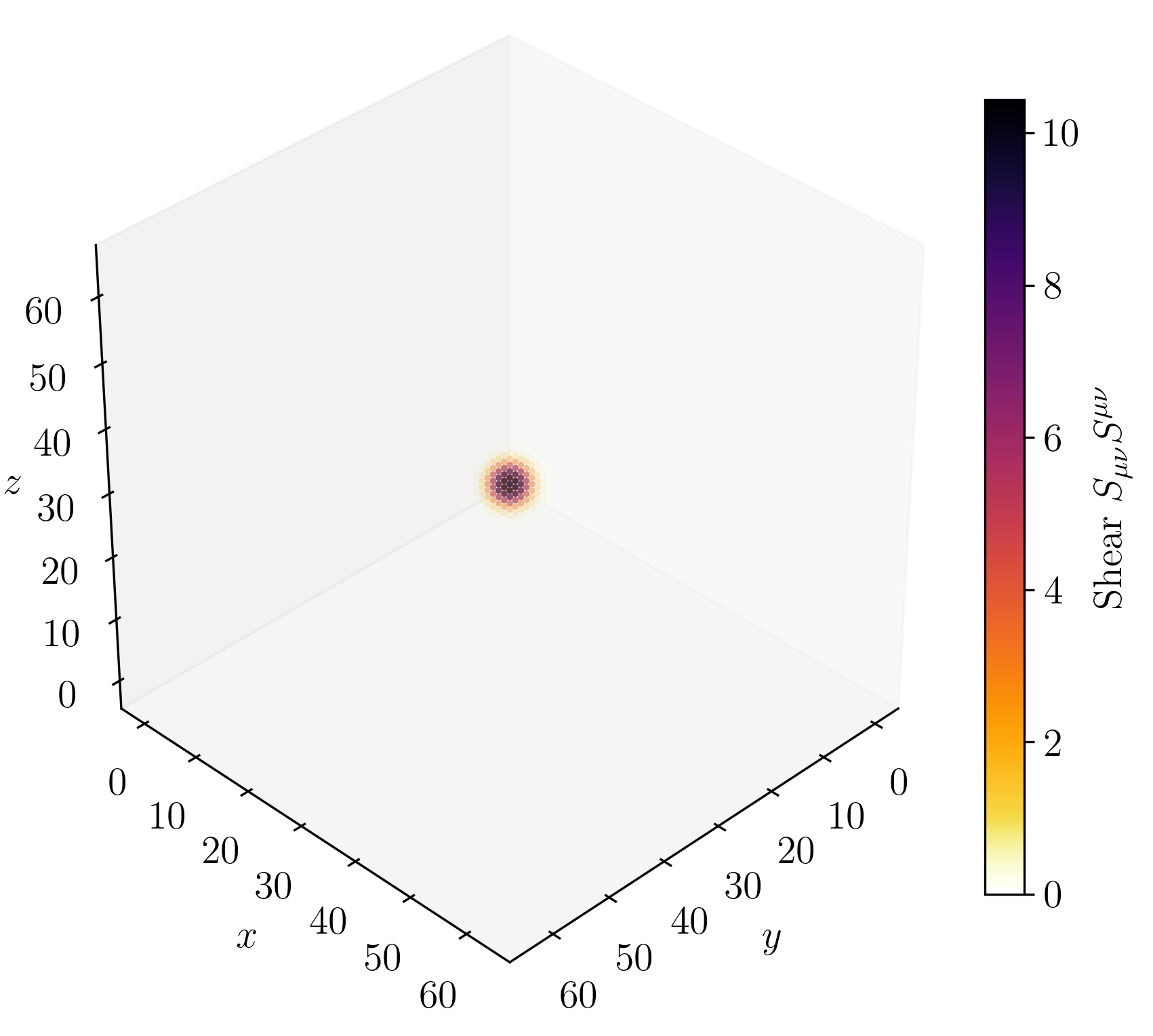
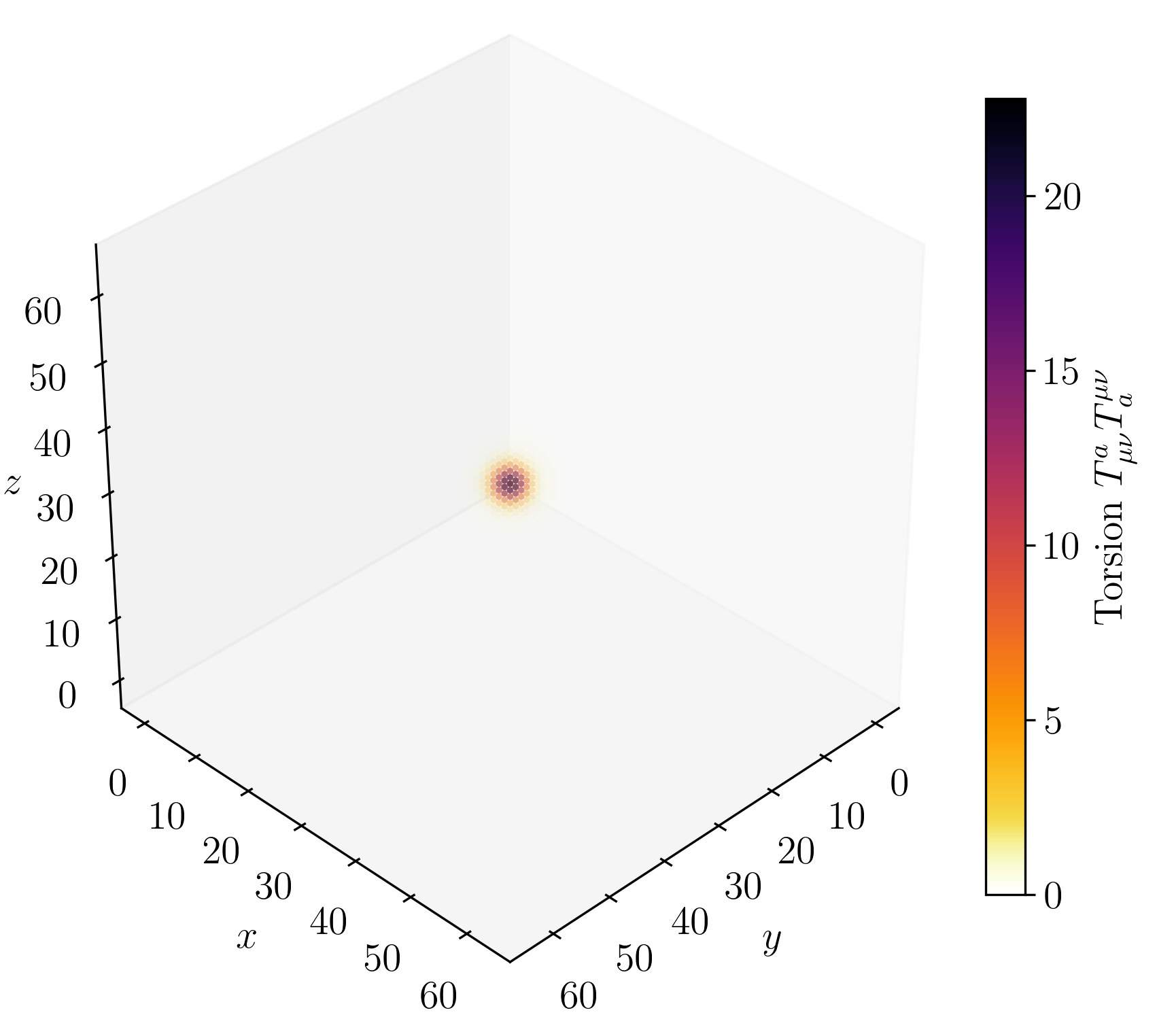
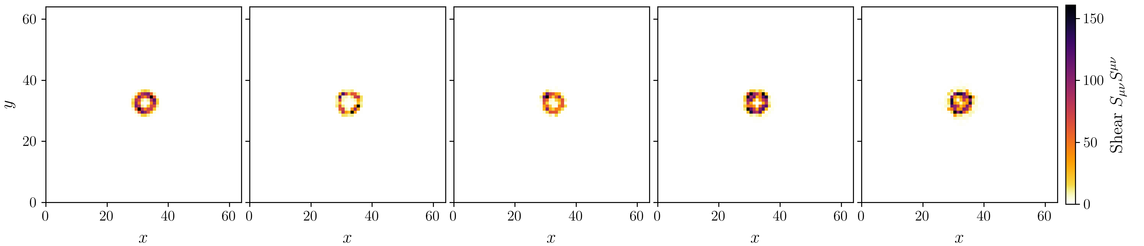
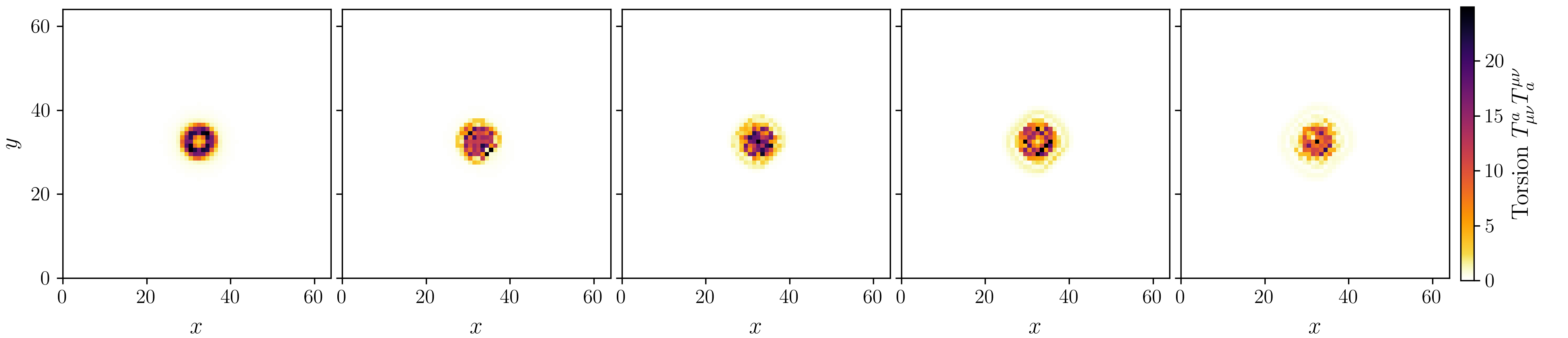
6.1 Charge-Carrying Solitons
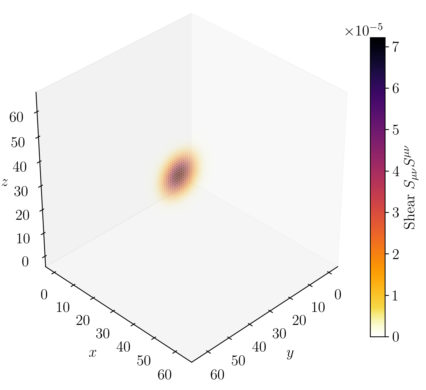
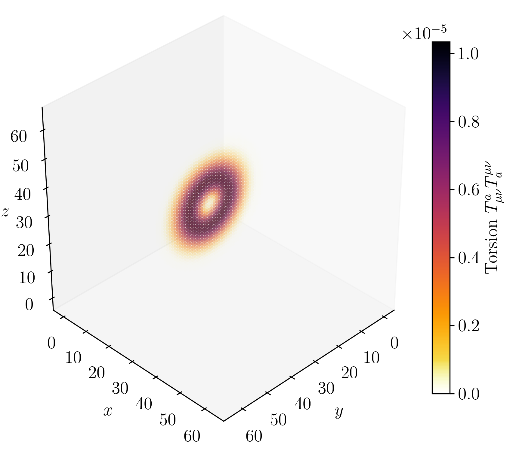
To seed a single charged soliton in the structured vacuum, we populate both dynamical fields on the lattice. Not only do both fields provide the soliton with mass and charge, but each also crucially balances the forces of the opposite field, allowing the soliton to oscillate in place without propagating.
For the displacement field, \(u_i\), we initialize a purely azimuthal vortex that falls off as \(u_\psi \propto \frac {1}{\rho ^2}\). This displacement vortex supplies a long-range Coulomb-like field and stabilises the core. The rotation field, \(e^{a}{}_{\mu }\), is the product of two smooth rotations about the radial unit vector \(\hat {n}\) and stores the spin-texture and the torsion monopole that gives rise to electric charge.
We define the soliton core radius as \(R_e\). Outside the core (\(\rho > R_e\)), we add a thin azimuthal halo,
\[ \textbf {u}(\rho ,\psi )\;=\;u_{0}\,\frac {R_e^{2}}{\rho ^{2}}\,\hat {e}_{\psi }, \qquad \hat {\psi }\;\equiv \;(-\sin \psi ,\cos \psi ,0), \]
which supplies the \(\frac {1}{\rho ^2}\) elastic strain required by the lowest-order field equation and ensures that the lattice Coulomb energy matches the continuum value once the system is let free to relax.
For every lattice site, we compute the distance \(\rho = |\textbf {x}-\textbf {x}_{c}|\) to the chosen center and the radial direction \(\textbf {n}\). We then apply two rotation matrices successively:
-
1. A hedgehog flip \(R_{\text {hedg}}(\rho ) = \exp (+\chi (\rho )\,\textbf {n}\cdot \textbf {J})\) with \(\chi (\rho )=\pi \operatorname {sech}(\frac {\rho }{R_e})\). This carries the tetrad smoothly from the identity at infinity to a \(180^{\circ }\) inversion at the origin and produces a net torsion charge \(q=+1\).
-
2. A half-spin twist \(R_{\text {spin}}(\rho ) = \exp (+\theta (\rho )\,\textbf {n}\cdot \textbf {J})\) with \(\theta (\rho )=\pi \left [1-\operatorname {tanh}(\frac {\rho }{R_e})\right ]\). This extra \(\text {SU}(2)\) half-turn endows the defect with the correct fermionic sign change under a \(2\pi \) rotation.
The stored frame is the composition of these two rotations, \(e=R_{\text {spin}}R_{\text {hedg}}\). Because both angles go to zero exponentially, \(e\) is exactly the vacuum frame outside a sphere of radius \(\approx 3R_{e}\); no high-\(k\) noise is introduced.
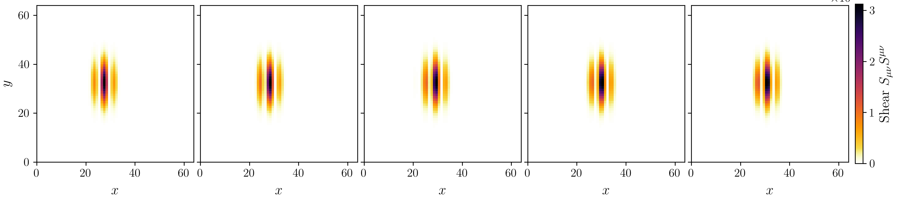
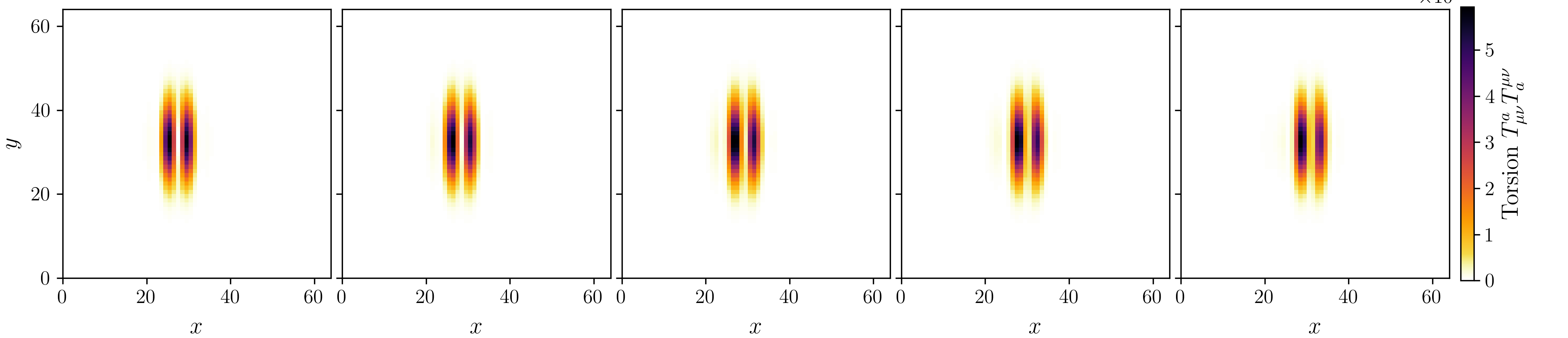
Figure 2 on page (page for fig. 2) shows 3D renderings of the initial state of shear and twist sectors and a cross-section of the \(z\)-axis at \(n=32\) every \(500\) simulation steps.
6.2 Propagating Waves
We encode a vector potential akin to magnetism in the displacement field \(u_i\) and a torsion field akin to electromagnetism in the rotation field \(e^{a}{}_{\mu }\). These two fields are then enveloped in a Gaussian wave-packet that travels in the \(+x\) direction.
We define a separable Gaussian with longitudinal coordinate \(\xi \equiv x-x_c\) and transverse coordinates \(\eta \equiv y-y_c,\;\zeta \equiv z-z_c\),
\[ \operatorname {env}(\xi ,\eta ,\zeta )\;=\;\exp \left (-\frac {\xi ^{2}}{2\sigma ^{2}_{x}}-\frac {\eta ^{2}}{2\sigma ^{2}_{y}}-\frac {\zeta ^{2}}{2\sigma ^{2}_{z}}\right ), \]
and a carrier phase \(\phi =k\xi \) with wave–number \(k=\frac {2\pi }{\lambda }\) and frequency \(\omega =c k, c \equiv \frac {\lambda _{T}}{\lambda {S}}\). Throughout we fix the propagation, electric and magnetic axes to
\[ \hat {\textbf {k}}\;=\;+\hat {x},\qquad \hat {\textbf {e}}\;=\;+\hat {y},\qquad \hat {\textbf {b}}\;=\;+\hat {z}\quad \left (\hat {\textbf {b}}\;=\;\hat {\textbf {k}}\times \hat {\textbf {e}}\right ). \]
The complementary shear component is taken along the magnetic axis,
\[ \textbf {u}(\textbf {x})\;=\;\frac {A_{0}}{k}\,\operatorname {env}\sin k\xi \,\hat {\textbf {b}}, \qquad \partial _{\xi }\textbf {u}\;=\;\frac {A_{0}}{k}\left (-\frac {\xi }{\sigma ^{2}_{x}}\operatorname {env}\sin k\xi +k\operatorname {env}\cos k\xi \right )\hat {\textbf {b}}, \]
and the canonical momentum is set to \(p_i=-c\,\partial _\xi u_i\) so that the linearised shear equation \(\partial _t u_i=p_i\) holds exactly at \(t=0\)
A small-angle rotation about the rank-1 generator \(\hat {\mathbf e}\otimes \hat {\mathbf k}^{\top }\) produces the twist sector. The rotation angle and its longitudinal derivative are
\[ \theta (\xi ,\eta ,\zeta )\;=\;\frac {A_{0}}{k}\,\operatorname {env}\cos k\xi ,\qquad \theta _{\xi }'\;=\;A_{0}\left (-\frac {\xi }{\sigma ^{2}_{x}}\operatorname {env}\cos k\xi -k\operatorname {env}\sin k\xi \right ). \]
Because \((e,u)\) and \((\omega ,p)\) are phased as above, the quadratic energy density
\[ \mathcal {E}\;=\;\lambda _{S}\,\frac {1}{2}\,\bigl |\nabla u\bigr |^{2}+\lambda _{T}\,\frac {1}{2}\,\bigl |\nabla T^{\hat {0}}\bigr |^{2}+\frac {1}{2}\left (\bigl |p\bigr |^{2}+\bigl |\omega \bigr |^{2}\right ) \]
is positive definite, localised by the Gaussian envelope, and splits equally between electric and magnetic sectors, reproducing the continuum Maxwell result to \(\order {A_0^2}\).
Similar to before, Figure 3 on page (page for fig. 3) shows 3D renderings of the initial state of shear and twist sectors and a cross-section of the \(z\)-axis at \(n=32\) every \(500\) simulation steps. Since the wave packet is symmetric about the \(x-\) and \(y\)-axes, we show a slice of the twist field at \(z=\frac {N}{2}\) as a representative view. The color gradient represents the displacement of the vector \(u_{i}\) and rotation of the frame \(e_i\) at each site, with higher contrast colors indicating larger displacements.
| Parameter | Natural | Simulation |
Provenance |
| \(\lambda _{S}\) | \(1/(32\pi G)\) | \(1.0\) |
Normalises the spin-2 kinetic term; fixes the code light–cone once \(\lambda _T=\lambda _1\). |
| \(\lambda _{T}\) | \(=\lambda _{1}\) | \(1.0\) |
Ensures photons propagate at the same speed as gravitons (\(c_T=c_S\)). |
| \(\lambda _{C}\) | \(\omega _{\mathrm {BD}}\) | \(10^{5}\) |
Brans–Dicke bound from Cassini tracking: \(\omega _{\mathrm {BD}}\gtrsim 4\times 10^{4}\) [32]. |
| \(\alpha _S\) | \(1/(16\pi G)=2\lambda _{1}\) | \(2.0\) |
Matches the cubic part of the teleparallel Einstein–Hilbert action. |
| \(\alpha _T\) | \(\displaystyle \frac {2\alpha ^2}{45,m_e^{4}}\sim 10^{-14}\lambda _{1}\) | \(10^{-14}\) |
Euler–Heisenberg one-loop value for low-energy QED; kept tiny so that QED non-linear optics is perturbative. |
| \(\alpha _{C}\) | \(\sim !10^{-120}M_{\rm Pl}^{4}\) | \(10^{-8}\) |
Toy dark-energy scale: tiny but large enough to resolve numerically. |
| \(\alpha _{H}\) | \(\le 10^{-6}\lambda _{1}\) | \(10^{-6}\) |
GW170817, GRB170817A arrival-time bound on \(|c_{\rm GW}-c_{\gamma }|\) [6]. |
| \(\alpha _{R}\) | \(\le 10^{-8}\lambda _{1}\) | \(10^{-8}\) |
Pulsar-timing array limit on running \(G\) (strain–dilaton mixing). |
| \(\alpha _{P}\) | \(\le 10^{-8}\lambda _{1}\) | \(10^{-8}\) |
Same order as \(\alpha _{\Sigma }\) to avoid excessive \(\sigma \)–torsion coupling. |
6.3 Cavity Standing Waves
The quartic action, Equation (12), predicts that shear and twist fields couple through the helixity invariant \(\alpha_{H}S^{\mu\nu}S_{\mu\nu}T^{\alpha}{}_{\rho\sigma}T_{\alpha}{}^{\rho\sigma}\). At quadratic order the two sectors evolve independently; the helixity term is the leading interaction that allows electromagnetic energy to drive gravitational displacements and vice versa. We test this prediction by simulating an electromagnetic standing wave inside a Gaussian cavity envelope and comparing two runs: one with the helixity coupling active (\(\alpha_{H}=\lambda_{1}\), boosted six orders of magnitude above the GW170817 bound for numerical visibility) and a control with \(\alpha_{H}=0\). Every other parameter is identical between the two runs.
We seed a transverse electromagnetic standing wave at wavelength \(\lambda=8\) lattice units, propagating along \(\hat{x}\) with electric polarisation along \(\hat{y}\) and magnetic displacement along \(\hat{z}\). The twist angle and transverse displacement are
\[ \theta(\xi)\;=\;2A_{0}\,\mathrm{env}(\xi,\eta,\zeta)\,\cos k\xi, \qquad u_{z}(\xi)\;=\;\frac{2A_{0}}{k}\,\mathrm{env}\,\sin k\xi, \]
with peak amplitude \(A_{0}=0.15\,\mathrm{rad}\) and a separable Gaussian envelope \(\mathrm{env}=\exp(-\xi^{2}/2\sigma_{x}^{2}-\eta^{2}/2\sigma_{y}^{2}-\zeta^{2}/2\sigma_{z}^{2})\) of widths \(\sigma_{x}=8,\;\sigma_{y}=\sigma_{z}=12\). All canonical momenta are set to zero, placing the standing wave at its maximum-amplitude turning point. Because a purely transverse wave produces zero diagonal strain (\(\mathrm{diag}(e^{\top}\nabla u)=0\)), the \(\nabla(T^{2})\cdot\mathrm{strain\_dir}\) channel in the shear equation of motion is inactive. To open this channel we add a small longitudinal breathing-mode seed,
\[ u_{x}(\xi)\;=\;\epsilon\,\frac{2A_{0}}{k}\,\mathrm{env}\,\sin k\xi, \qquad \epsilon = 0.01, \]
which provides the diagonal strain needed for the helixity coupling to transfer energy from the twist sector into the shear sector.
Both simulations evolve the identical initial condition for 1000 RK4 time steps on a \(64^{3}\) periodic lattice. The difference field \(\Delta\phi\equiv\phi_{\alpha_{H}=\lambda_{1}}-\phi_{\alpha_{H}=0}\) isolates the contribution of the helixity coupling from the linear dynamics, which are shared by both runs. We observe four distinct coupling signatures in the final state.
Longitudinal displacement. Figure 4 (top) shows the longitudinal displacement \(u_{x}\) along the propagation axis at \(y=z=N/2\). The coupled and control profiles are visually identical at the scale of the full field, but their difference \(\Delta u_{x}\) (bottom panel) reveals a coherent oscillatory pattern with RMS amplitude \(1.6\times 10^{-5}\), localised within the Gaussian cavity envelope. The 2D slice at \(z=N/2\) in Figure 5 confirms that the coupling signature inherits the standing-wave spatial structure and vanishes outside the envelope.
Harmonic generation. The Fourier power spectrum of \(\Delta u_{x}\) (Figure 6) peaks at the cavity fundamental \(k=1/\lambda\) and exhibits a secondary peak near \(3k\). The third harmonic arises because the helixity force term \(2\alpha_{H}\nabla(T^{2})\cdot\mathrm{strain\_dir}\) is quadratic in the torsion field: the product \(\sin(2k\xi)\cos(k\xi)\) generates both \(k\) and \(3k\) spatial harmonics. This nonlinear frequency conversion is absent from the control run and is a direct fingerprint of the quartic cross-coupling.
Torsion backreaction. The coupling is bidirectional. The shear-dependent force on the twist sector, \(2\alpha_{H}S^{2}\cdot\mathrm{torque}\), modifies the torsion field by \(33.7\%\) (RMS \(\Delta T^{2}=7.4\times 10^{-5}\)) relative to the uncoupled control. The torsion difference is largest at the \(T^{2}\) peaks, consistent with the \(S^{2}T^{2}\) structure of the helixity invariant: the backreaction is strongest where both fields are intense.
Gravitational-wave polarisation. The transverse-traceless projection of the strain tensor yields two gravitational-wave polarisations, \(h_{+}\) and \(h_{\times}\). Figure 7 plots the transverse-plane-averaged RMS of each polarisation as a function of lattice site along the propagation axis. Both modes trace the standing-wave envelope, with \(h_{+}\) and \(h_{\times}\) shifted by half a wavelength—reflecting the quarter-wave offset between the displacement and twist profiles of the cavity mode. The coupling-induced change (bottom panel) reveals a mild asymmetry: \(\Delta\,\mathrm{RMS}(h_{+})\simeq 7.0\times 10^{-7}\) while \(\Delta\,\mathrm{RMS}(h_{\times})\simeq 4.2\times 10^{-7}\). The preferential modification of the plus mode reflects the standing-wave geometry: the torsion gradient \(\nabla(T^{2})\) is aligned along \(\hat{x}\) and sources diagonal strain (\(h_{+}\)) more efficiently than off-diagonal strain (\(h_{\times}\)). A circularly polarised or isotropic cavity configuration would produce a different polarisation mixture, providing a direct experimental handle for identifying helixity-mediated gravitational radiation.
Taken together, these four signatures—coherent displacement growth, third-harmonic generation, torsion backreaction, and polarised gravitational-wave emission—constitute a numerical demonstration that the helixity cross-coupling in the structured vacuum quartic action produces measurable bidirectional energy transfer between the electromagnetic and gravitational sectors.
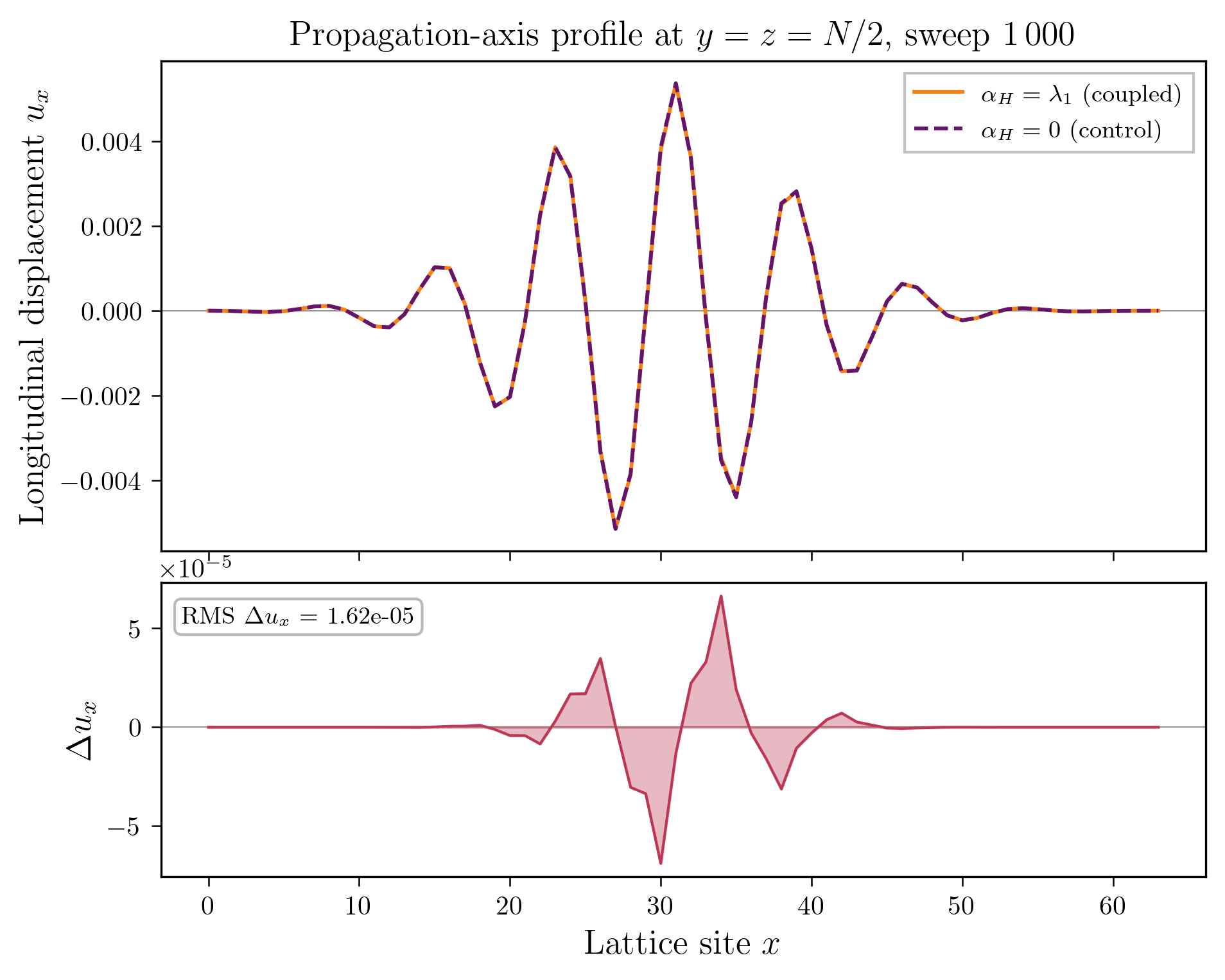
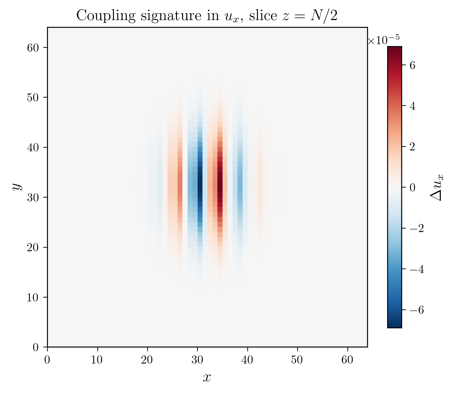
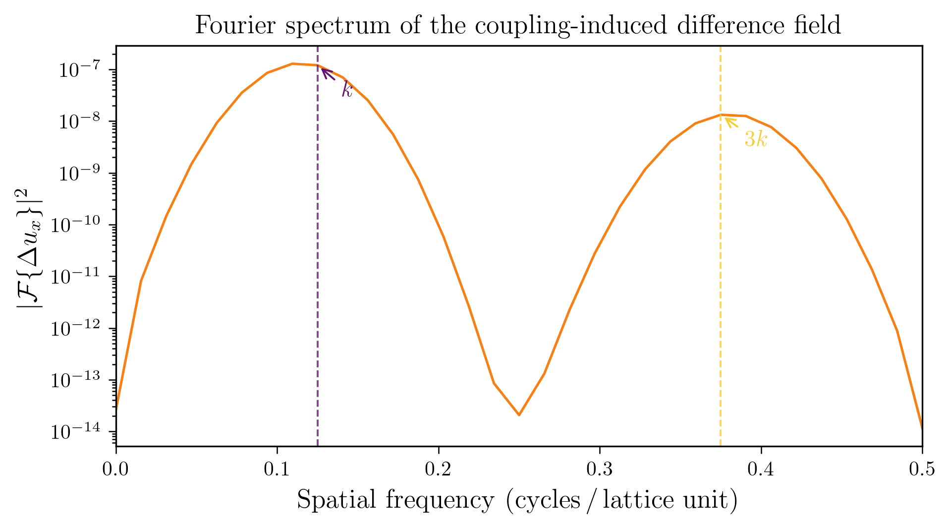
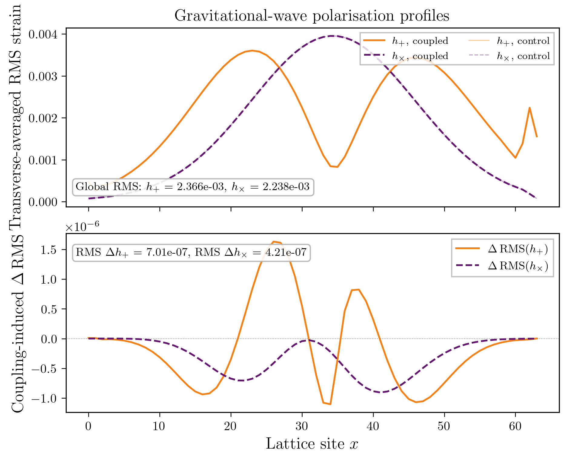
7 Conclusions
We began this work by posing the question, ”What emergent behavior arises if the vacuum of space is not empty but has structure?” To help answer this question, we endowed the vacuum with a geometric structure
consisting of a displacement field, a rotation field, and a scale field. We then found that through successive derivation and elimination of unphysical interactions between these fields, our model naturally led to the emergence of
relativistic gravity from its pure shear interactions, electromagnetism from its pure twist interactions, and a scalar-tensor field through its scale interactions. A potentially fruitful area of future work is to explore the cross-coupling
between these fields—if they are measurable then they hint at hitherto undetected physics.We demonstrated numerically that the helixity cross-coupling between these fields produces measurable bidirectional energy transfer between the electromagnetic and gravitational sectors—coherent displacement growth, third-harmonic generation, torsion backreaction, and polarised gravitational-wave emission—confirming that the quartic action predicts hitherto undetected physics that is, in principle, testable. We also release a free and open source simulator that allows for curious readers to explore the structured vacuum model and its emergent
behavior in a numerical setting. It is our hope that this work encourages a curious and inquisitive view toward the vacuum of space and inspires further research into physics that may be hidden in seemingly empty space.
A Invariant Candidates
Below we enumerate every two- and four-derivative candidate that can be formed from the declared first-derivative blocks
\[ S_{\mu \nu }\equiv \nabla _{(\mu }u_{\nu )},\qquad T^{a}{}_{\mu \nu }\equiv 2\,\mathcal D_{[\mu }e^{a}{}_{\nu ]},\qquad s_{\mu }\equiv \nabla _{\mu }\sigma , \]
together with \(g_{\mu \nu },\,\eta _{ab},\,\epsilon _{\mu \nu \rho \sigma }\).
For each discarded term we give the reason, using the criteria from Sections 4.1 and 5.1:
-
b boundary / total divergence (integral independence)
-
0 identically zero (symmetry/antisymmetry)
-
e proportional to a quadratic EOM (field redefinition)
-
p/t violates the parity/time-reversal projection
-
r redundant / algebraically dependent (Schouten identities, index symmetries, \(2\)-form identities)
-
g pure-gauge spin-connection artifact (we work with flat \(\omega \), \(R[\omega ]=0\))
-
t trace moved into \(\sigma \) (use \(\sigma =\ln |e|\simeq S^{\mu }{}_{\mu }+\mathcal O(S^{2})\) so isotropic dilation is carried by \(\sigma \))
A.1 Quadratic (Two-Derivative) Invariants
The three kept terms are \(S_{\mu \nu }S^{\mu \nu }\), \(T^{a}{}_{\mu \nu }T_{a}{}^{\mu \nu }\), and \(s_{\mu }s^{\mu }\). All other candidates fall into one of the cases below.
A.1.1 Terms linear in a first derivative
-
• \(\nabla _{\mu }u^{\mu }=S^{\mu }{}_{\mu }\). b, integrates to a boundary; also t, isotropic part carried by \(\sigma \).
-
• \(\nabla _{\mu }\sigma \) alone. b, surface term.
-
• \(T^{a}{}_{\mu \nu }\) alone. 0, cannot form a scalar without \(\epsilon \) (which would be p/t).
A.1.2 Built from \(\partial u\)
-
• Full gradients \(\nabla _{\mu }u_{\nu }\nabla ^{\mu }u^{\nu }\) and \(\nabla _{\mu }u_{\nu }\nabla ^{\nu }u^{\mu }\) decompose into \(S_{\mu \nu }S^{\mu \nu }+A_{\mu \nu }A^{\mu \nu }\) with \(A_{\mu \nu }\) antisymmetric. \(A_{\mu \nu }A^{\mu \nu }\) is r/g; keep only \(S_{\mu \nu }S^{\mu \nu }\).
-
• Trace terms such as \((S^{\mu }{}_{\mu })^{2}\) or \(S^{\mu }{}_{\mu }S_{\rho \sigma }S^{\rho \sigma }\) are t.
A.1.3 Built from \(T^{a}{}_{\mu \nu }\)
Let \(T^{\rho }{}_{\mu \nu }\equiv e_{a}{}^{\rho }T^{a}{}_{\mu \nu }\). In \(4\)D the classical invariants are
\[ \mathcal I_{1}=T_{\rho \mu \nu }T^{\rho \mu \nu },\quad \mathcal I_{2}=T_{\rho \mu \nu }T^{\mu \rho \nu },\quad \mathcal I_{3}=T_{\mu }T^{\mu },\quad T_{\mu }\equiv T^{\nu }{}_{\mu \nu }. \]
-
• Keep \(\mathcal I_{1}\).
-
• \(\mathcal I_{2},\mathcal I_{3}\) are r and e.
-
• Parity-odd \(\epsilon ^{\mu \nu \rho \sigma }T^{a}{}_{\mu \nu }T_{a\,\rho \sigma }\) is p/t.
-
• Nieh–Yan density is b/g for \(R[\omega ]=0\).
A.1.4 Cross terms among \(S,T,s\)
-
• \(S_{\mu \nu }T^{a\,\mu \nu }\) is 0.
-
• \(S_{\mu \nu }s^{\mu }s^{\nu }\) has three derivatives, not quadratic.
-
• \(T^{a}{}_{\mu \nu }\epsilon ^{\mu \nu \rho \sigma }s_{\rho }s_{\sigma }\) is p/t and not quadratic.
A.1.5 \(\sigma \)-sector with second derivatives
-
• \((\Box \sigma )\) or \((\nabla _{\mu }\nabla _{\nu }\sigma )\) at quadratic order are e/r via parts and \(\Box \sigma =0\).
A.2 Quartic (Four-Derivative) Invariants
The kept basis in Eq. (12) is:
\[ \begin {aligned} &\text {(i) } \alpha _{S}\left (S_{\mu \nu }S^{\nu \rho }S_{\rho \sigma }S^{\sigma \mu }-S_{\mu \nu }S^{\mu \nu }S_{\rho \sigma }S^{\rho \sigma }\right ),\\ &\text {(ii) } \frac 14\alpha _{T}\left (T^{a}\!\cdot T_{a}\right )^{2},\quad \text {(iii) } \alpha _{C}\,(s^{2})^{2},\\ &\text {(iv) } \alpha _{H}S^{\mu \nu }S_{\mu \nu }\,T^{a}{}_{\rho \sigma }T_{a}{}^{\rho \sigma },\\ &\text {(v) } \alpha _{R}S^{\mu \nu }S_{\mu \nu }\,s^{2},\quad \text {(vi) } \alpha _{P}T^{a}{}_{\rho \sigma }T_{a}{}^{\rho \sigma }\,s^{2}. \end {aligned} \]
A.2.1 Pure-shear \(S^{4}\)
Two non-trace contractions:
\[ \mathcal S_{1}=\mathrm {Tr}[S^{4}],\qquad \mathcal S_{2}=(\mathrm {Tr}[S^{2}])^{2}. \]
Traceful variants are t. Keep \(\mathcal S_{1}-\mathcal S_{2}\). The orthogonal combination is r.
A.2.2 Pure-twist \(T^{4}\)
With \(X^{a}_{\mu \nu }=T^{a}{}_{\mu \nu }\):
\[ (X^{a}\!\cdot \!X_{a})^{2},\quad (X^{a}\!\cdot \!\widetilde X_{a})^{2},\quad (X^{a}\!\cdot \!X_{a})(X^{b}\!\cdot \!\widetilde X_{b}). \]
Keep \((X^{a}\!\cdot \!X_{a})^{2}\). The other two are p/t. Index-shuffle quartics are r.
A.2.3 Pure-scale \(s^{4}\)
Only \((s^{2})^{2}\) is independent. Second-derivative forms are e/r.
A.2.4 Shear–twist \(S^{2}T^{2}\)
\[ \mathcal H_{1}=S_{\mu \nu }S_{\rho \sigma }T^{a\,\mu \rho }T_{a}{}^{\nu \sigma },\quad \mathcal H_{2}=S_{\mu }{}^{\rho }S_{\nu \rho }T^{a\,\mu \sigma }T_{a}{}^{\nu }{}_{\sigma },\quad \mathcal H_{3}=S_{\mu \nu }S_{\rho \sigma }T^{a\,\mu \nu }T_{a}{}^{\rho \sigma },\quad \mathcal H_{4}=S_{\mu \nu }S_{\rho \sigma }T^{a\,\mu \rho }\widetilde T_{a}{}^{\nu \sigma }. \]
\(\mathcal H_{3}\) is 0, \(\mathcal H_{4}\) is p/t, \(\mathcal H_{1,2}\) reduce to kept helixity plus boundary (r/e).
A.2.5 Shear–scale \(S^{2}s^{2}\)
\(\mathcal R_{1}=S_{\mu \nu }S^{\mu \nu }s^{2}\) (kept), \(\mathcal R_{2}=S_{\mu }{}^{\rho }S_{\nu \rho }s^{\mu }s^{\nu }\) is e/r.
A.2.6 Twist–scale \(T^{2}s^{2}\)
\(\mathcal P_{1}=T^{a}{}_{\rho \sigma }T_{a}{}^{\rho \sigma }s^{2}\) (kept), \(\mathcal P_{2}=T^{a}{}_{\mu \rho }T_{a\,\nu }{}^{\rho }s^{\mu }s^{\nu }\) is e/r.
A.2.7 Mixed with \(\epsilon \)
Examples: \(S_{\mu \nu }S_{\rho \sigma }T^{a\,\mu \rho }\widetilde T_{a}{}^{\nu \sigma }\), \(T^{a}\!\cdot \!\widetilde T_{a}S^{2}\), \((T^{a}\!\cdot \!\widetilde T_{a})^{2}\), etc. are p/t.
A.2.8 Quartics with derivatives on the blocks
Forms like \(\nabla _{\alpha }S_{\mu \nu }\nabla ^{\alpha }S^{\mu \nu }\), \(\nabla _{\alpha }T^{a}{}_{\mu \nu }\nabla ^{\alpha }T_{a}{}^{\mu \nu }\), \(s^{\mu }\nabla _{\mu }s^{2}\) are r/e.
A.2.9 “Cross-sector squares” of vanishing quadratics
Squares of quadratics that are 0 or p/t remain excluded.
In summary, at two derivatives the only nontrivial scalars are \(S^{2}\), \(T^{2}\), and \(s^{2}\). At four derivatives, up to boundaries and quadratic EOMs, the complete parity-even, local, Lorentz-covariant, index-algebra-unique set built from these blocks is exactly the six terms kept in Eq. (12).
References
-
[1] E. Tiesinga et al., “CODATA recommended values of the fundamental physical constants: 2018,” Rev. Mod. Phys. 93, 025010 (2021).
-
[2] D. M. Pozar, Microwave Engineering, 4th ed. (Wiley, 2011), §6.4.
-
[3] H. Padamsee, RF Superconductivity for Accelerators, 2nd ed. (Wiley-VCH, 2009), Table 2.2.
-
[4] A. Gurevich, “Superconducting radio-frequency fundamentals for particle accelerators,” Rev. Accel. Sci. Tech. 10, 1–51 (2017).
-
[5] C.,M. Will, The Confrontation between General Relativity and Experiment, Living Rev. Relativity 17 (2014) 4.
-
[6] B.P. Abbott et al. (LIGO/Virgo), GW170817: Observation of Gravitational Waves from a Binary Neutron Star Inspiral, Phys. Rev. Lett. 119 (2017) 161101.
-
[7] A. D. Sakharov, “Vacuum quantum fluctuations in curved space and the theory of gravitation,” Sov. Phys. Dokl. 12, 1040 (1968).
-
[8] M. Visser, “Sakharov’s induced gravity: a modern perspective,” Mod. Phys. Lett. A 17, 977 (2002).
-
[9] T. Jacobson, “Thermodynamics of spacetime: the Einstein equation of state,” Phys. Rev. Lett. 75, 1260 (1995).
-
[10] E. P. Verlinde, “On the origin of gravity and the laws of Newton,” JHEP 04 (2011) 029.
-
[11] W. G. Unruh, “Experimental black-hole evaporation?,” Phys. Rev. Lett. 46, 1351 (1981).
-
[12] C. Barceló, S. Liberati, and M. Visser, “Analogue gravity,” Living Rev. Relativ. 8, 12 (2005).
-
[13] M. A. Levin and X.-G. Wen, “String-net condensation: a physical mechanism for topological phases,” Phys. Rev. B 71, 045110 (2005).
-
[14] M. Hermele, M. P. A. Fisher, and L. Balents, “Pyrochlore photons: the U(1) spin liquid in a \(S\!=\!1/2\) frustrated magnet,” Phys. Rev. B 69, 064404 (2004).
-
[15] K. S. Stelle, “Renormalization of higher-derivative quantum gravity,” Phys. Rev. D 16, 953 (1977).
-
[16] A. A. Starobinsky, “A new type of isotropic cosmological model without singularity,” Phys. Lett. B 91, 99 (1980).
-
[17] NANOGrav Collaboration (Z. Arzoumanian et al.), “The NANOGrav 12.5-yr data set: search for a gravitational-wave background,” Astrophys. J. Lett. 905, L34 (2020).
-
[18] NANOGrav Collaboration (G. Agazie et al.), “The NANOGrav 15-yr data set: evidence for a gravitational-wave background,” Astrophys. J. Lett. 951, L8 (2023).
-
[19] J. Antoniadis et al., “The International Pulsar Timing Array evidence for an isotropic gravitational-wave background,” Astron. Astrophys. 677, A24 (2023).
-
[20] T. Robson, N. J. Cornish, and C. Liu, “The construction and use of LISA sensitivity curves,” Class. Quantum Grav. 36, 105011 (2019).
-
[21] S. Kawamura et al., “The Japanese space gravitational wave antenna: DECIGO,” Class. Quantum Grav. 28, 094011 (2011).
-
[22] R. Abbott et al. (LIGO Scientific, Virgo, and KAGRA Collaborations), “Prospects for observing and localizing gravitational-wave transients with Advanced LIGO, Advanced Virgo and KAGRA during the fourth observing run,” Living Rev. Relativ. 26, 1 (2023).
-
[23] M. Maggiore, “Stochastic backgrounds of gravitational waves,” Phys. Rep. 331, 283 (2000).
-
[24] A. M. Cruise and R. M. J. Ingley, “A prototype gravitational wave detector for 100 MHz,” Class. Quantum Grav. 23, 6185 (2006).
-
[25] Z. Li and R. M. L. Baker, “MHz- to GHz-band gravitational-wave detection using coupled superconducting resonators,” Phys. Rev. D 108, 042005 (2023).
-
[26] C. Caprini and D. G. Figueroa, “Cosmological backgrounds of gravitational waves,” Class. Quantum Grav. 35, 163001 (2018).
-
[27] V. Domcke, M. Geller, and N. Schwieterman, “Fundamental physics with high-frequency gravitational waves,” JHEP 03 (2022) 055.
-
[28] K. Schmitz, “New sensitivities to primordial gravitational waves,” Universe 7, 373 (2021).
-
[29] M. E. Gertsenshtein, “Wave resonance of light and gravitational waves,” Sov. Phys. JETP 14, 84 (1962).
-
[30] H. Padamsee, RF Superconductivity: Science, Technology, and Applications (Wiley-VCH, Weinheim, 2017).
-
[31] M. Goryachev and M. E. Tobar, “Gravitational wave detection with high frequency phonon trapping acoustic cavities,” Phys. Rev. D 92, 044043 (2015).
-
[32] C. M. Will, “The confrontation between general relativity and experiment,” Living Rev. Relativ. 17, 4 (2014).
-
[33] B. Bertotti, L. Iess, and P. Tortora, “A test of general relativity using radio links with the Cassini spacecraft,” Nature 425, 374 (2003).
-
[34] U. D. Jentschura, “Lamb shift in a laser-modified vacuum,” Phys. Rev. A 84, 012505 (2011).
-
[35] K. Yagi and L. C. Stein, “Black-hole perturbation theory in the frequency domain,” Class. Quantum Grav. 33, 054001 (2016).
-
[36] N. Aghanim et al. (Planck Collaboration), “Planck 2018 results. VI. Cosmological parameters,” Astron. Astrophys. 641, A6 (2020).
-
[37] R. Abbott et al. (LIGO Scientific and Virgo Collaborations), “Tests of general relativity with binary black holes from the second LIGO–Virgo gravitational-wave transient catalog,” Phys. Rev. D 103, 122002 (2021).
-
[38] E. Zavattini et al. (PVLAS Collaboration), “Improved limits on optical rotation and vacuum birefringence using a high-finesse Fabry–Pérot cavity,” Phys. Rev. D 104, 092005 (2021).
-
[39] A. K. Harding and D. Lai, “Physics of strongly magnetized neutron stars,” Rep. Prog. Phys. 69, 2631 (2006).
-
[40] M. S. Pshirkov, D. B. Blaschke, and J. C. Fabris, “Constraints on the stochastic background of high-frequency gravitational waves,” Phys. Rev. D 82, 083008 (2010).
-
[41] R. Abbott et al. (LIGO Scientific, Virgo and KAGRA Collaborations), “High-frequency gravitational wave search using data from Advanced LIGO and Virgo’s third observing run,” Phys. Rev. D 104, 102004 (2021).
-
[42] R. Bähre et al., “Any Light Particle Search II — Technical design report,” JINST 8, T09001 (2013); updated status 2019, DESY-20-021.
-
[43] J. F. Donoghue, “General relativity as an effective field theory: the leading quantum corrections,” Phys. Rev. D 50, 3874 (1994).
-
[44] M. Reuter and F. Saueressig, Quantum Gravity and the Functional Renormalization Group (Cambridge Univ. Press, 2019).
-
[45] G. E. Volovik, The Universe in a Helium Droplet (Oxford Univ. Press, 2003).
-
[46] I. T. Drummond and S. J. Hathrell, "QED vacuum polarization in a background gravitational field and its effect on the velocity of photons," Phys. Rev. D 22, 343 (1980).
Changelog
Copyright © 2025–2026 Justin J. Meza. This work is licensed under a Creative Commons Attribution 4.0 International License (CC BY 4.0). To view a copy of this license, visit http://creativecommons.org/licenses/by/4.0/ or send a letter to Creative Commons, PO Box 1866, Mountain View, CA 94042, USA.